정보
-
업무명 : 직달 일사량 자료를 이용한 일조량 산출 및 비교 분석
-
작성자 : 이상호
-
작성일 : 2020-01-06
-
설 명 :
-
수정이력 :
내용
[특징]
-
직달 일사량 및 일조량을 이해하기 위해서 가시화 및 비교 분석이 요구되며 이 프로그램은 이러한 목적을 달성하기 위한 소프트웨어
[기능]
-
직달 일사량을 이용하여 일조량 산출 및 비교 분석
[활용 자료]
-
자료명 : 단파 복사 및 장파 복사 자료
-
자료 종류 : 직달 일사량, 일조량
-
확장자 : dat
-
기간 : 2012년 10월 11일 - 2017년 07월 05일
-
자료 해상도 : 1초 샘플링하여 1분 평균
-
제공처 : 강릉원주대 생명대학 2호관 옥상 (복사 관측소)
-
자세한 정보는 아래 링크 참조
[Fortran, Gnuplot, ShellScript] 기상 자료를 이용한 통계 분석 및 가시화
정보 업무명 : 기상 자료를 이용한 통계 분석 및 가시화 작성자 : 이상호 작성일 : 2019-08-31 설 명 : 수정이력 : 내용 [특징] 기상 자료의 특성을 파악하기 위해 통계 분석 및 가시화 도구가 필요하며 이 프로그..
shlee1990.tistory.com
[자료 처리 방안 및 활용 분석 기법]
-
없음
[사용법]
-
입력 자료를 동일 디렉터리 위치
-
소스 코드를 실행 (Rscript
Retrieval_and_Comparison_Analysis_of_Sunshine_Duration_Using_Pyrheliometer_Data.R)
-
가시화 결과를 확인
[사용 OS]
-
Windows 10
[사용 언어]
-
R v3.6.2
-
R Studio v1.2.5033
소스 코드
[명세]
-
전역 설정
-
최대 10 자리 설정
-
메모리 해제
-
# Set Option
options(digits = 10)
memory.limit(size = 9999999999999)
-
라이브러리 읽기
# Library Load
library(tidyverse)
library(data.table)
library(lubridate)
library(timeDate)
library(extrafont)
library(colorRamps)
library(RColorBrewer)
-
파일 읽기
# File Read
dfData = fread("total.dat")
colnames(dfData) = c("st", "year", "month", "day", "hour", "minute", "press", "geo", "temp", "dewpt", "dir", "wspd", NA, NA, NA)

dplyr::glimpse(dfData)
-
함수 선언
# Function Load
fnStatResult = function(xAxis, yAxis) {

   if (length(yAxis) > 0) {
      nSlope = coef(lm(yAxis ~ xAxis))[2]
      nInterp = coef(lm(yAxis ~ xAxis))[1]
      nMeanX = mean(xAxis, na.rm = TRUE)
      nMeanY = mean(yAxis, na.rm = TRUE)
      nSdX = sd(xAxis, na.rm=  TRUE)
      nSdY = sd(yAxis, na.rm = TRUE)
      nNumber = length(yAxis)
      nBias = mean(xAxis - yAxis, na.rm = TRUE)
      nRelBias = (nBias / mean(yAxis, na.rm = TRUE))*100.0
      # nRelBias = (nBias / mean(xAxis, na.rm = TRUE)) * 100.0
      nRmse = sqrt(mean((xAxis - yAxis)^2, na.rm = TRUE))
      nRelRmse = (nRmse / mean(yAxis, na.rm = TRUE)) * 100.0
      # nRelRmse = (nRmse / mean(xAxis, na.rm = TRUE)) * 100.0
      nR = cor(xAxis, yAxis)
      nMeanDiff = mean(xAxis - yAxis, na.rm = TRUE)
      nSdDiff = sd(xAxis - yAxis, na.rm = TRUE)
      nPerMeanDiff = mean((xAxis - yAxis) / yAxis, na.rm = TRUE) * 100.0
      nPvalue = cor.test(xAxis, yAxis)$p.value

      return( c(nSlope, nInterp, nMeanX, nMeanY, nSdX, nSdY, nNumber, nBias, nRelBias, nRmse, nRelRmse, nR, nMeanDiff, nPerMeanDiff, nPerMeanDiff, nPvalue) )
   }
}
-
단파복사 자료 읽기
# Shortwave Radiation File Read
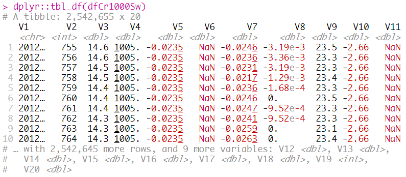
dfCr1000Ver1 = data.table::fread("20121011-20140623.dat", header = FALSE, sep = ",", skip = 4)
dfCr1000Ver2 = data.table::fread("20140624-20151217.dat", header = FALSE, sep = ",", skip = 4)
dfCr1000Ver3 = data.table::fread("CR1000_Table1.dat", header = FALSE, sep = ",", skip = 4)
dfCr1000Sw = dplyr::bind_rows(dfCr1000Ver1, dfCr1000Ver2, dfCr1000Ver3)
dplyr::tbl_df(dfCr1000Sw)
-
장파복사 자료 읽기
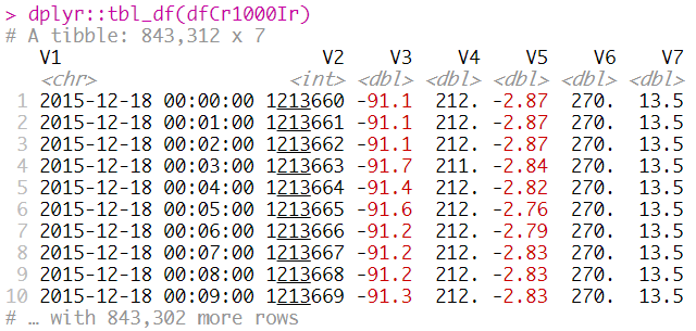
# Longwave Radiation File Read
dfCr1000Ir = fread("CR1000_2_Table1.dat", header = FALSE, sep = ",", skip = 4)

dplyr::tbl_df(dfCr1000Ir)
-
Data Frame 설정
-
장파복사 (dfCr1000Ir) 좌측 조인
-
연-월-일 시:분:초를 날짜 형태로 변환
-
# Set Data Frame
dfData = dfCr1000Sw %>%
dplyr::left_join(dfCr1000Ir, by = "V1") %>%
dplyr::mutate(
dtDateTime = readr::parse_datetime(V1, format = "%Y-%m-%d %H:%M:%S")
, nYear = lubridate::year(dtDate)
, nMonth = lubridate::month(dtDate)
, nDay = lubridate::day(dtDate)
, nHour = lubridate::hour(dtDate)
, nMinute = lubridate::minute(dtDate)
, nSec = lubridate::second(dtDate)
, nLastDayInMonth = lubridate::day(timeDate::timeLastDayInMonth(format(dtDate, "%Y%m%d"), format = "%Y%m%d", zone = "Asia/Seoul"))
, xranYmdHms =
nYear + ((nMonth - 1) / 12.0) + ((nDay - 1) / (12.0 * nLastDayInMonth)) + (nHour / (12.0 * nLastDayInMonth * 24.0))
+ (nMinute / (12.0 * nLastDayInMonth * 24.0 * 60.0))
+ (nSec / (12.0 * nLastDayInMonth * 24.0 * 60.0 * 60.0))
, xranYmd = nYear + ((nMonth - 1) / 12.0) + ((nDay - 1) / (12.0 * nLastDayInMonth))
)
# Set Coloum Name
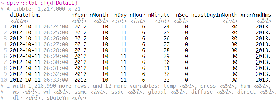
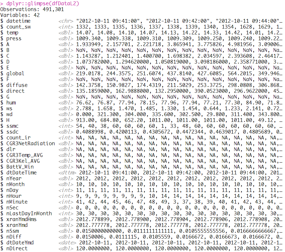
colnames(dfData) = c("datetime", "count_sw", "temp", "press", "A", "B", "C", "D", "E", "global", "F", "diffuse", "direct", "G", "hum", "ws", "wd", "H", "ssmc", "ssdc", "count_ir", "CGR3NetRadiation", "dlr", "CGR3Temp_AVG", "CGR3Kel_AVG", "BattV_Min", "dtDateTime", "nYear", "nMonth", "nDay", "nHour", "nMinute", "nSec", "nLastDayInMonth", "xranYmdHms", "xranYmd")
# count(관측 기록 횟수), temp(외부 온도), press(관측소 기압), Awm(전천일사), Cwm(산란일사),
# Dwm(직달일사), Hum(상대 습도), ws(풍속), wd(풍향), ssmc(분누적 일조 : 횟수), ssdc(일누적 일조 : 시간)
# CGR3NetRadiation (순복사), dlr(하향장파복사), CGR3Temp_AVG(섭씨 온도), CGR3Kel_AVG(켈빈 온도)
dplyr::glimpse(dfData)

-
Filter Data Frame 설정
-
제외할 사례 선정
-
# Set Filter Data Frame
dfFilterDate = data.frame(
   sDateYm = c(
      "2016-03"
      , "2016-06"
      , "2016-09"
      , "2016-12"
      )
)
-
Data Frame를 통해 L1 전처리
-
열 선택 (dtDateTime, nYear, nMonth, nDay, nHour, nMinute, nSec, nLastDayInMonth, xranYmdHms, temp, press, hum, ws, wd, ssmc, ssdc, global, diffuse, direct, dlr)
-
사례 제외 그리고 전천/산란/직달 일사량 최대값 및 최소값 설정
-
# L1 Processing Using Data Frame
dfDataL1 = dfData %>%
   dplyr::select(dtDateTime, nYear, nMonth, nDay, nHour, nMinute, nSec, nLastDayInMonth, xranYmdHms, temp, press, hum, ws, wd, ssmc, ssdc, global, diffuse, direct, dlr) %>%
   dplyr::mutate(sDateYm = format(dtDateTime, "%Y-%m")) %>%
   dplyr::filter(
      ! sDateYm %in% dfFilterDate$sDateYm
      , dplyr::between(global, 0, 4000)
      , dplyr::between(diffuse, 0, 4000)
      , dplyr::between(direct, 0, 4000)
      )

dplyr::tbl_df(dfDataL1)
-
L1 자료를 통해 출력
# Write Using L1 Data Frame
data.table::fwrite(
   dfDataL1
   , sep = ","
   , file = "OUTPUT/dfDataL1.csv"
   , append = FALSE
   , row.names = FALSE
   , col.names = TRUE
   , dateTimeAs = "write.csv"
   , na = NA
)

-
Filter Data Frame 설정
-
제외할 사례 선정
-
# Set Data Frame
dfFilterDate = data.frame(
   sDateYmd = c(
      "2013-05-16"
      , "2013-07-07"
      , "2013-09-23"
      , "2014-03-04"
      , "2014-07-08"
      , "2014-09-15"
      , "2015-03-01"
      , "2015-03-02"
      , "2015-04-22"
      , "2015-08-19"
      , "2015-08-31"
      , "2017-02-14"
      , "2017-02-15"
      , "2017-02-16"
      , "2017-02-17"
      , "2017-02-18"
      , "2017-02-19"
      , "2017-02-20"
      , "2017-02-21"
      , "2017-02-22"
      , "2017-02-23"
      , "2017-02-24"
      , "2017-02-25"
      , "2017-02-26"
      , "2017-02-27"
      , "2017-02-28"
      , "2017-02-29"
      , "2017-03-01"
      , "2017-03-02"
      , "2017-03-03"
      , "2017-03-04"
      , "2017-03-05"
      , "2017-03-06"
      , "2017-03-07"
      , "2017-06-02"
      )
)
-
Data Frame 자료를 통해 L2 전처리
-
매 분마다 직달 일사량 (nDirect)이 120 Wm-2 이하일 경우에 대해 0-60으로 선형 내삽
-
관측소 번호/년/월/기압에 따라 평균, NA 개수, Not NA 개수, 정상화율 계산
-
# L2 Processing Using Data Frame
dfDataL2 = dfData %>%
   dplyr::mutate(
      nSsm = ssmc / 3600.0
      , nDiff = ssdc - lag(ssdc)
      , dtDateYmd = as.Date(dtDateTime)
      , nDirect = dplyr::case_when(
         direct > 120 ~ 120
         , TRUE ~ direct
         )
      ) %>%
   dplyr::filter(
      dplyr::between(nHour, 09, 15)
      , ssmc > 0
      , nDiff > 0
      , nSsm > 0
      , nDirect > 0
      , ! dtDateYmd %in% as.Date(dfFilterDate$sDateYmd)
      ) %>%
   dplyr::mutate(
      nDirectSsmc = approx(c(0, 120), c(0, 60), xout = nDirect)$y
      )

dplyr::glimpse(dfDataL2)
-
L2 자료를 통해 L3 전처리
-
연/월/일에 따라 직달 일사량으로부터 일조량, 일조계로부터 일조량, 두 자료의 차이, 최대 직달 일사량, 최대 전천 일사량, 자료 개수를 계산
-
자료 개수 및 시간에 대해 각각 0-420개 및 2013-2016년으로 설정
-
# L3 Processing Using Data Frame L2
dfDataL3 = dfDataL2 %>%
dplyr::group_by(nYear, nMonth, nDay, xranYmd) %>%
dplyr::summarise(
nSumSsm = sum(ssmc, na.rm = TRUE) / 3600.0
, nSumDirectSsm = sum(nDirectSsmc, na.rm = TRUE) / 3600.0
, nSumDiff = sum(nDiff, na.rm = TRUE)
, nMaxDirect = max(direct, na.rm = TRUE)
, nMaxGlobal = max(global, na.rm = TRUE)
, iNumber = n()
) %>%
dplyr::filter(
dplyr::between(iNumber, 0, 420)
, dplyr::between(xranYmd, 2013, 2016)
)
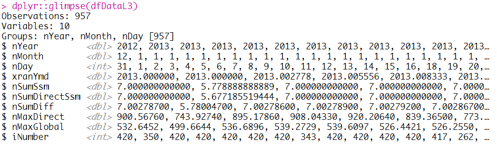
dplyr::glimpse(dfDataL3)
-
산점도를 위한 초기 설정
# Set Value for Visualization
xAxis = dfDataL3$nSumDirectSsm
yAxis = dfDataL3$nSumSsm

xcord = 0.25
ycord = seq(7.75, 0, -0.5)
cbSpectral = rev(RColorBrewer::brewer.pal(11, "Spectral"))
font = "Palatino Linotype"
nVal = fnStatResult(xAxis, yAxis)  ;  sprintf("%.3f", nVal)
-
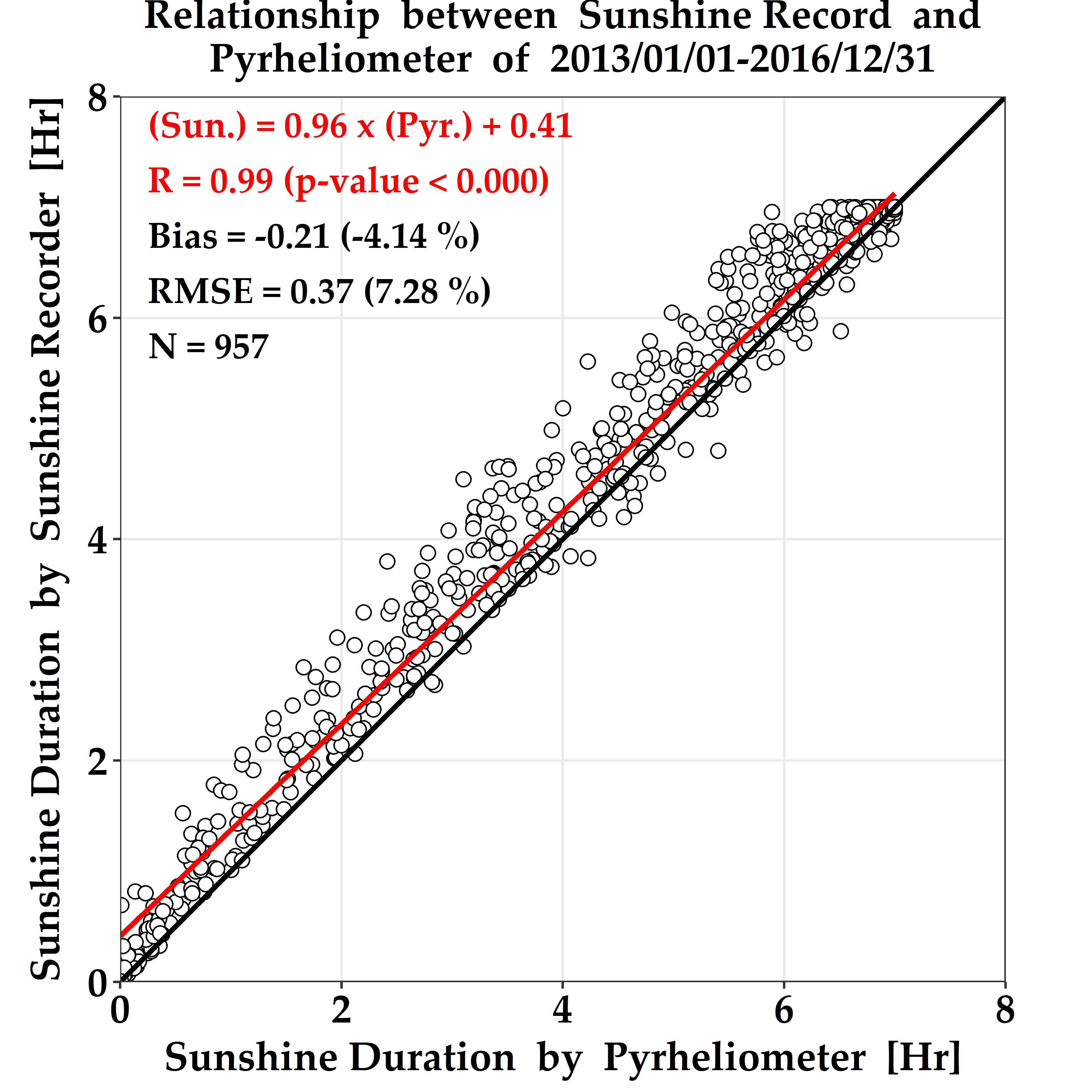
ggplot2를 이용한 산점도
# Scatterplot Using ggplot2
ggplot() +
   coord_fixed(ratio = 1) +
   theme_bw() +
   geom_point(data = dfDataL3, aes(xAxis, yAxis), shape = 21, colour = "black", fill = "white", size = 2.5) +
   annotate("text", x = xcord, y = ycord[1], label = paste0("(Sun.) = ", sprintf("%.2f", nVal[1])," x (Pyr.) + ", sprintf("%.2f", nVal[2])), size = 5, hjust = 0, color = "red", fontface = "bold", family = font) +
   annotate("text", x = xcord, y = ycord[2], label = paste0("R = ", sprintf("%.2f", nVal[12]), " (p-value < ", sprintf("%.3f", nVal[16]), ")"), size = 5, hjust = 0, color = "red", family = font, fontface = "bold") +
   annotate("text", x = xcord, y = ycord[3], label = paste0("Bias = ", sprintf("%.2f", nVal[8]), " (", sprintf("%.2f", nVal[9])," %)"), parse = FALSE, size = 5, hjust = 0, family = font, fontface = "bold") +
   annotate("text", x = xcord, y = ycord[4], label = paste0("RMSE = ", sprintf("%.2f",nVal[10]), " (", sprintf("%.2f", nVal[11])," %)"), parse = FALSE, size = 5, hjust = 0, family = font, fontface = "bold") +
   annotate("text", x = xcord, y = ycord[5], label = paste0("N = ", format(nVal[7], big.mark = ",", scientific = FALSE)), size = 5, hjust = 0, color = "black", family = font, fontface = "bold") +
   geom_abline(intercept = 0, slope = 1, linetype = 1, color = "black", size = 1.0) +
   stat_smooth(data = dfDataL3, aes(xAxis, yAxis), method = "lm", color = "red", se = FALSE) +
   scale_x_continuous(minor_breaks = seq(0, 8, 2), breaks=seq(0, 8, 2),  expand = c(0, 0), limits = c(0, 8)) +
   scale_y_continuous(minor_breaks = seq(0, 8, 2), breaks=seq(0, 8, 2),  expand = c(0, 0), limits = c(0, 8)) +
   labs(
      title = "Relationship  between  Sunshine Record  and\n  Pyrheliometer  of  2013/01/01-2016/12/31"
      , y = expression(paste(bold("Sunshine Duration  by  Sunshine Recorder  [Hr]")))
      , x = expression(paste(bold("Sunshine Duration  by  Pyrheliometer  [Hr]")))
      , fill = "Count"
      ) +
   theme(
      plot.title=element_text(face = "bold", size = 16, color="black", hjust = 0.5)
      , axis.title.x = element_text(face = "bold", size = 16, colour = "black")
      , axis.title.y = element_text(face = "bold", size = 16, colour = "black", angle = 90)
      , axis.text.x = element_text(face = "bold", size = 16, colour = "black")
      , axis.text.y = element_text(face = "bold", size = 16, colour = "black")
      , legend.title=element_text(face = "bold", size = 14, colour = "black")
      , legend.position = c(0, 1), legend.justification = c(0, 0.96)
      , legend.key=element_blank()
      , legend.text=element_text(size = 14, face = "bold")
      , legend.background=element_blank()
      , text=element_text(family = font)
      , plot.margin=unit(c(0, 8, 0, 0), "mm")
      ) +
   ggsave(filename = paste0("FIG/Sunshine Duration.png"), width = 6, height = 6, dpi = 600)
-
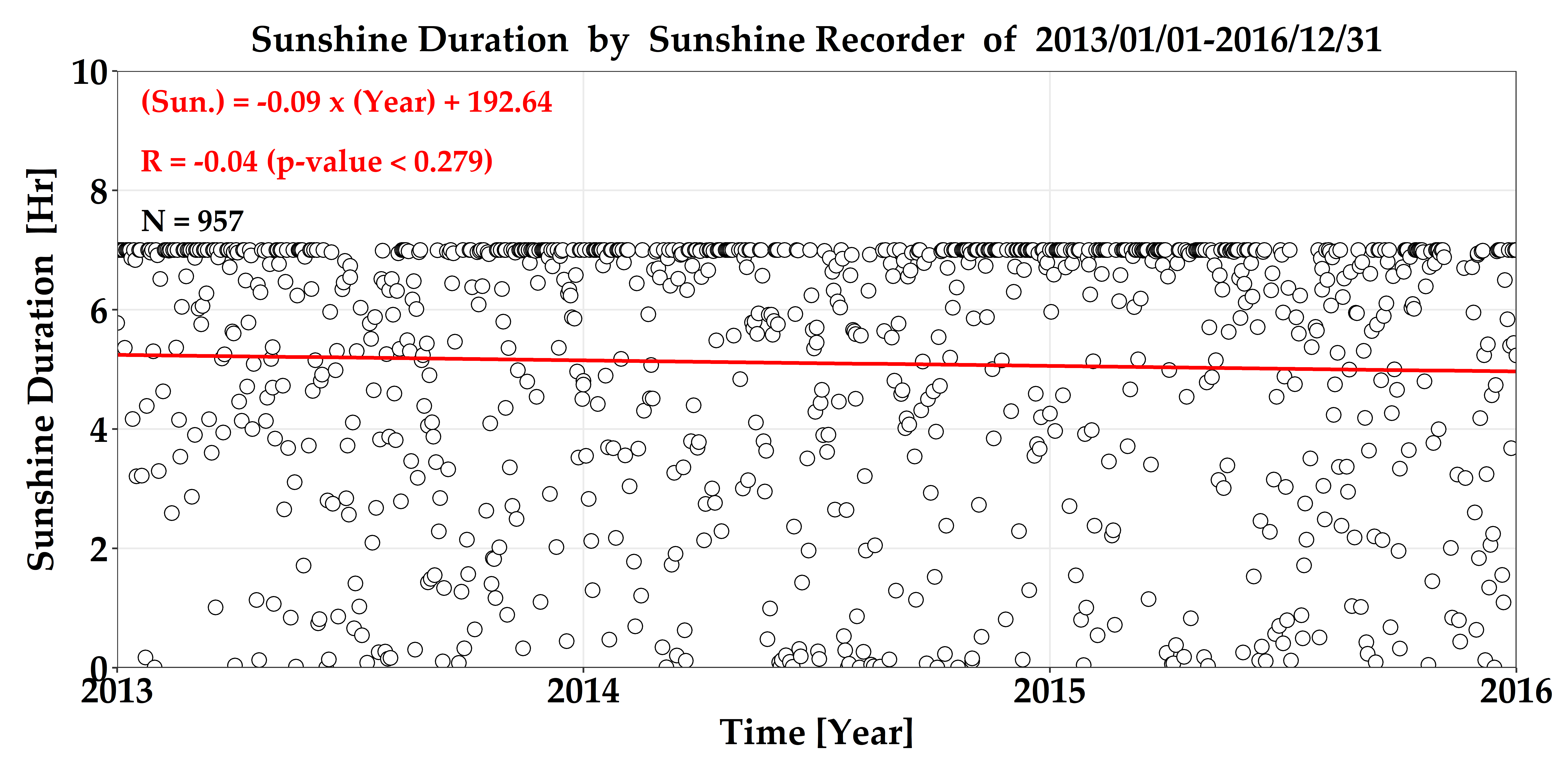
시계열을 위한 초기 설정
# Set Value for Visualization
xAxis = dfDataL3$xranYmd

yAxis = dfDataL3$nSumSsm
yAxis = dfDataL3$nSumDirectSsm

nVal = fnStatResult(xAxis, yAxis)  ;  sprintf("%.3f", nVal)
xcord = 2013.05
ycord = seq(9.5, 0, -1.0)
-
ggplot2를 이용한 시계열
# Time series Using ggplot2
ggplot() +
   # coord_fixed(ratio = 1) +
   theme_bw() +
   geom_point(data = dfDataL3, aes(xAxis, yAxis), shape = 21, colour = "black", fill = "white", size = 3.5) +
   annotate("text", x = xcord, y = ycord[1], label = paste0("(Sun.) = ", sprintf("%.2f", nVal[1])," x (Year) + ", sprintf("%.2f", nVal[2])), size = 6, hjust = 0, color = "red", fontface = "bold", family = font) +
   annotate("text", x = xcord, y = ycord[2], label = paste0("R = ", sprintf("%.2f", nVal[12]), " (p-value < ", sprintf("%.3f", nVal[16]), ")"), size = 6, hjust = 0, color = "red", family = font, fontface = "bold") +
   annotate("text", x = xcord, y = ycord[3], label = paste0("N = ", format(nVal[7], big.mark = ",", scientific = FALSE)), size = 6, hjust = 0, color = "black", family = font, fontface = "bold") +
   geom_abline(intercept = 0, slope = 1, linetype = 1, color = "black", size = 1.0) +
   stat_smooth(data = dfDataL3, aes(xAxis, yAxis), method = "lm", color = "red", se = FALSE) +
   scale_x_continuous(minor_breaks = seq(2013, 2016, 1), breaks = seq(2013, 2016, 1),  expand=c(0, 0), limits=c(2013,  2016)) +
   scale_y_continuous(minor_breaks = seq(0, 10, 2), breaks = seq(0, 10, 2),  expand = c(0, 0), limits=c(0, 10)) +
   labs(
      # title = "Sunshine Duration  by  Sunshine Recorder  of  2013/01/01-2016/12/31"
      title = "Sunshine Duration  by  Pyrheliometer  of  2013/01/01-2016/12/31"
      , x = expression(paste(bold("Time [Year]")))
      , y = expression(paste(bold("Sunshine Duration  [Hr]")))
      , fill = NULL
      ) +
   theme(
      plot.title = element_text(face = "bold", size = 20, color = "black", hjust = 0.5)
      , axis.title.x = element_text(face = "bold", size = 20, colour = "black")
      , axis.title.y = element_text(face = "bold", size = 20, colour = "black", angle = 90)
      , axis.text.x = element_text(face = "bold", size = 20, colour = "black")
      , axis.text.y = element_text(face = "bold", size = 20, colour = "black")
      , legend.title = element_text(face = "bold", size = 12, colour = "black")
      , legend.position = c(0, 1), legend.justification = c(0, 0.9)
      , legend.key = element_blank()
      , legend.text = element_text(size=12, face="bold")
      , legend.background = element_blank()
      , text=element_text(family = font)
      , plot.margin = unit(c(5, 10, 5, 5), "mm")
      ) +
   # ggsave(filename = paste0("FIG/Sunshine Duration_Time_sun.png"), width = 12, height = 6, dpi = 600)
   ggsave(filename = paste0("FIG/Sunshine Duration_Time_pyr.png"), width = 12, height = 6, dpi = 600)

[전체]
참고 문헌
[논문]
- 없음
[보고서]
- 없음
[URL]
- 없음
문의사항
[기상학/프로그래밍 언어]
- sangho.lee.1990@gmail.com
[해양학/천문학/빅데이터]
- saimang0804@gmail.com


최근댓글