

정보
-
업무명 : 소프트웨어 개발
-
작성자 : 이상호
-
작성일 : 2019-12-31
-
설 명 :
-
수정이력 :
내용
[특징]
-
새해 경자년에 해돋이 (일출) 시간을 이해하기 위해서 가시화가 요구되며 이 프로그램은 이러한 목적을 달성하기 위한 소프트웨어
[기능]
-
기상 관측소 정보를 이용한 전국 해돋이 (일출) 시각 맵핑
-
각 관측소에 대한 2019년 일출/일몰 시간 시계열
[활용 자료]
-
자료명 : 기상 관측소 정보
-
자료 종류 : 관측소 지점 번호, 경도, 위도, 관측소명
[자료 처리 방안 및 활용 분석 기법]
-
없음
[사용법]
- 입력 자료를 동일 디렉터리 위치
- 소스 코드를 실행 (Rscript Visualization_and_Preprocessing_Using_Weather_Station_Data_for_Sunrise_and_Sunset_Times.R)
- 가시화 결과 확인
[사용 OS]
-
Window 10
[사용 언어]
-
R v 3.6.2
-
R Studio v1.2.5033
소스 코드
[명세] 해돋이 (일출) 시각 맵핑
-
전역 설정
-
자리수 설정
-
영문 설정
-
# Set Option
options(digits = 10)
Sys.setlocale("LC_TIME", "english")
-
라이브러리 읽기
# Library Load
library(data.table)
library(suncalc)
library(tidyverse)
library(scales)
library(sf)
library(gstat)
library(sp)
library(metR)
library(colorRamps)
library(ggrepel)
library(extrafont)
library(timeDate)
-
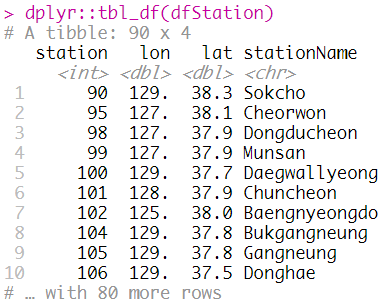
기상 관측소 정보 읽기
# File Read
dfStation = fread("INPUT/Station_Information.dat", sep = "\t", header = FALSE, skip = 1)
colnames(dfStation) = c("station", "lon", "lat", "stationName")

dplyr::tbl_df(dfStation)
-
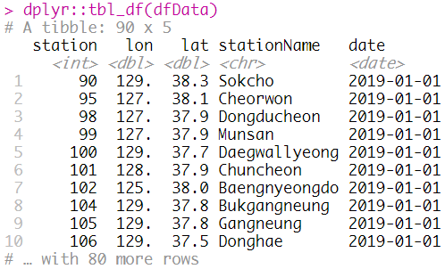
Data Frame 형태로 초기화
# Set Data Frame
dfData = dfStation %>%
   dplyr::mutate(date = lubridate::ymd("2019-01-01"))

dplyr::tbl_df(dfData)
-
Data Frame를 통해 L1 전처리
-
getSunlightTimes 함수를 통해 일출 (해돋이) 및 일몰 시간 계산
-
dfDataL1을 기준으로 기상 관측소 정보를 좌측 조인
-
xranYmdHms, xranHms 변수 초기화
-
# L1 Processing Using Data Frame
dfDataL1 = getSunlightTimes(
   data = dfData
   , keep = c("sunrise", "sunriseEnd", "sunset", "sunsetStart")
   ,  tz = "Asia/Seoul"
) %>%
   dplyr::left_join(dfStation, by=c("lat" = "lat", "lon" = "lon")) %>%
   dplyr::mutate(
      dtDate = sunrise
      , nYear = lubridate::year(dtDate)
      , nMonth = lubridate::month(dtDate)
      , nDay = lubridate::day(dtDate)
      , nHour = lubridate::hour(dtDate)
      , nMinute = lubridate::minute(dtDate)
      , nSec = lubridate::second(dtDate)
      , nLastDayInMonth = lubridate::day(timeDate::timeLastDayInMonth(format(dtDate, "%Y%m%d"), format = "%Y%m%d", zone = "Asia/Seoul"))
      , xranYmdHms =
         nYear + ((nMonth - 1) / 12.0) + ((nDay - 1) / (12.0 * nLastDayInMonth))
         + (nHour / (12.0 * nLastDayInMonth * 24.0))
         + (nMinute / (12.0 * nLastDayInMonth * 24.0 * 60.0))
         + (nSec / (12.0 * nLastDayInMonth * 24.0 * 60.0 * 60.0))
      , xranHms =
         nHour + (nMinute / 60.0) + (nSec / (60.0 * 60.0))
      )

dplyr::tbl_df(dfDataL1)
dplyr::glimpse(dfDataL1)


-
맵핑을 위한 설정
# Set Value for Visualization
cbMatlab =  colorRamps::matlab.like(11)
font = "Palatino Linotype"
mapKor = read_sf("INPUT/gadm36_KOR_shp/gadm36_KOR_1.shp")
mapPrk = read_sf("INPUT/gadm36_PRK_shp/gadm36_PRK_1.shp")
mapJpn = read_sf("INPUT/gadm36_JPN_shp/gadm36_JPN_1.shp")

spData = dfDataL1
coordinates(spData) = ~lon + lat

# plot(spData)

-
기상 관측소 정보를 통해 전처리
-
내삽을 위한 위/경도 설정
-
신규 격자 (spNewData)에 대해 "역거리 가중치 (IDW)" 공간 내삽 수행
-
# Processing Using Station Data
dfStationData = data.frame(
   nLat = spData$lat
   , nLon = spData$lon
   , sStationName  = as.character(spData$stationName)
)

# Min/Max Longitude of the Interpolation Area
xRange = as.numeric(c(124, 132))

# Min/Max Latitude of the Interpolation Area
yRange = as.numeric(c(33, 39))

# Expand Points to Grid
spNewData = expand.grid(
   x = seq(from = xRange[1], to = xRange[2], by = 0.1)
   , y = seq(from = yRange[1], to = yRange[2], by = 0.1)
)

coordinates(spNewData) = ~ x + y
gridded(spNewData) = TRUE

# Apply IDW Model for the Data
spDataL1 = gstat::idw(formula = xranHms ~ 1, locations = spData, newdata = spNewData)
-
L1을 통해 L2 전처리
# L2 Processing Using L1 Data Frame
dfDataL2 = spDataL1 %>%
   as.data.frame() %>%
   dplyr::rename(
      nLon = x
      , nLat = y
      , nVal = var1.pred
   ) %>%
   dplyr::mutate(isLand = metR::MaskLand(nLon, nLat, mask = "world")) %>%
   dplyr::filter(isLand == TRUE)

dplyr::tbl_df(dfDataL2)

-
L2 자료를 이용한 맵핑
-
해돋이 (일출) 시각에 대한 등고선
-
기상 관측소 정보 기입
-
남한/북한/일본 Shp
-
# Map Visualization Using ggplot2
ggplot() +
   coord_fixed(ratio = 1.1) +
   theme_bw() +
   geom_tile(data = dfDataL2, aes(x = nLon, y = nLat, fill = nVal)) +
   geom_point(data = dfStationData, aes(x = nLon, y = nLat), colour = "black", size= 5, alpha = 0.3, show.legend = FALSE) +
   geom_text_repel(data = dfStationData, aes(x = nLon, y = nLat, label = sStationName, colour=sStationName), point.padding = 0.25, box.padding = 0.25,  nudge_y = 0.1, size = 4, colour = "black", family = font) +
   geom_contour2(data = dfDataL2, aes(x = nLon, y = nLat, z = nVal), color = "red", alpha = 0.75, breaks = seq(7.5, 8.0, 0.05), show.legend = TRUE) +
   geom_text_contour(data = dfDataL2, aes(x = nLon, y = nLat, z = nVal), stroke = 0.2, breaks = seq(7.5, 8.0, 0.05), show.legend = TRUE) +
   scale_fill_gradientn(colours = cbMatlab, limits=c(7.5, 8), breaks = seq(7.5, 8.0, 0.25), na.value = cbMatlab[length(cbMatlab)], labels = c("7.50 (07:30)", "7.75 (07:45)" ,"8.00 (08:00)")) +
   geom_sf(data = mapKor, color = "black", fill = NA) +
   geom_sf(data = mapPrk, color = "black", fill = NA) +
   geom_sf(data = mapJpn, color = "black", fill = NA) +
   metR::scale_x_longitude(expand = c(0, 0), breaks = seq(124, 132, 2), limits = c(124, 132)) +
   metR::scale_y_latitude(expand = c(0, 0), breaks = seq(32, 40, 1), limits = c(33, 39)) +
   labs(x = ""
        , y = ""
        , fill = ""
        , colour = ""
        , title  = ""
        ) +
   theme(
      plot.title = element_text(face = "bold", size = 18, color = "black")
      , axis.title.x = element_text(face = "bold", size = 18, colour = "black")
      , axis.title.y = element_text(face = "bold", size=18, colour = "black", angle = 90)
      , axis.text.x = element_text(face = "bold", size=18, colour = "black")
      , axis.text.y = element_text(face = "bold", size=18, colour = "black")
      , legend.position = c(1, 1.03)
      , legend.justification = c(1, 1)
      , legend.key = element_blank()
      , legend.text = element_text(size = 14, face = "bold")
      , legend.title = element_text(face = "bold", size = 14, colour = "black")
      , legend.background=element_blank()
      , text=element_text(family = font)
      , plot.margin = unit(c(0, 8, 0, 0), "mm")
      ) +
   ggsave(filename = paste0('FIG/SunRise.png'), width = 8, height = 10, dpi = 600)
[명세] 해돋이 (일출) 시각 시계열
-
Data Frame 형태로 초기화
# Set Data Frame
dtDate = seq(lubridate::ymd("2019-01-01"), lubridate::ymd("2020-01-01"), by = "1 day")

for (iCount in 1:length(dtDate)) {

   dfTmp = dfStation %>%
      mutate(date = dtDate[iCount])

   if (iCount == 1) {
      dfTimeData = tibble::add_column(dfTmp)
   } else {
      dfTimeData = bind_rows(dfTimeData, dfTmp)
   }
}

dplyr::tbl_df(dfTimeData)
-
Data Frame를 통해 L1 전처리
-
getSunlightTimes 함수를 통해 일출 (해돋이) 및 일몰 시간 계산
-
dfDataL1을 기준으로 기상 관측소 정보를 좌측 조인
-
dfTimeDataL1 = getSunlightTimes(
   data = dfTimeData
   , keep = c("sunrise", "sunriseEnd", "sunset", "sunsetStart")
   , tz = "Asia/Seoul"
   ) %>%
   dplyr::left_join(dfStation, by=c("lat" = "lat", "lon" = "lon")) %>%
   dplyr::mutate(
      dtDate = as.POSIXct(date) - lubridate::hours(9)
      , dtSunrise = sunrise - dtDate
      , dtSunriseEnd = sunriseEnd - dtDate
      , dtSunset =  sunset - dtDate
      , dtSunsetStart = sunsetStart - dtDate
      )

dplyr::glimpse(dfTimeDataL1)

-
시계열을 위한 설정
-
폰트 설정
-
# Set Value for Visualization
font = "Palatino Linotype"
-
L1 자료를 이용한 시계열
-
2019년 1월 1일부터 2020년 1월 1일까지 하루 간격으로 해돋이 (일출) 및 일몰 시각에 대한 선 그래프
-
동/서/남해에 대한 대표 도시 (강릉, 인천, 부산) 선정
-
# Time series Visualization Using ggplot2
for (iCount in 1:nrow(dfStation)) {

   sStationName = as.character(dfStation[iCount, 4])
   sSaveFilePathName = paste0("FIG/Sunrise_and_Sunset_", sStationName, ".png")

   dfTimeDataL2 = dfTimeDataL1 %>%
      dplyr::filter(stationName == sStationName) %>%
      dplyr::arrange(date)

   dplyr::tbl_df(dfTimeDataL2)

   ggplot(data = dfTimeDataL2, aes(x = dtDate, ymin = dtSunrise, ymax = dtSunset)) +
      theme_bw() +
      geom_ribbon(fill = "#FDE725FF", alpha = 0.8) +
      scale_x_datetime(breaks = seq(min(dfTimeDataL2$dtDate), max(dfTimeDataL2$dtDate), "month"), expand = c(0, 0), labels = date_format("%b-%d\n%Y", tz = "Asia/Seoul"), minor_breaks = NULL) +
      scale_y_continuous(limits = c(4, 22), breaks = seq(4, 22, 4), expand = c(0, 0), minor_breaks = NULL) +
      labs(
         x = "Date [Month-Day Year]",
         y = "Sunrise and Sunset [Hour]",
         title = sprintf("Sunrise and Sunset for %s\n%s ", sStationName
                         , paste0(range(dfTimeData$date), sep = " ", collapse = "to "))
         ) +
      theme(
         panel.background = element_rect(fill = "#180F3EFF")
         , panel.grid = element_line(colour = "grey", linetype = "dashed")
         , plot.title = element_text(hjust = 0.5, face = "bold", size = 18, color = "black")
         , axis.title.x = element_text(face = "bold", size = 18, colour = "black")
         , axis.title.y = element_text(face = "bold", size = 18, colour = "black", angle = 90)
         , axis.text.x = element_text(angle = 45, hjust = 1, face = "bold", size = 18, colour="black")
         , axis.text.y = element_text(face = "bold", size = 18, colour = "black")
         , text = element_text(family = font)
         , plot.margin = unit(c(5, 10, 5, 5), "mm")
         ) +
      ggsave(filename = sSaveFilePathName, width = 12, height = 8, dpi = 600)
}
-
강릉
-
일출 시작/종료 : 07시 40분 55초 - 07시 44분 01초
-
일몰 시간/종료 : 17시 13분 33초 - 17시 16분 39초
-
-
인천
-
일출 시작/종료 : 07시 49분 14초 - 07시 52분 18초
-
일몰 시간/종료 : 17시 23분 24초 - 17시 26분 29초
-

-
부산
-
일출 시작/종료 : 07시 33분 14초 - 07시 36분 11초
-
일몰 시간/종료 : 17시 20분 15초 - 17시 23분 12초
-

[전체]
참고 문헌
[논문]
- 없음
[보고서]
- 없음
[URL]
- 없음
문의사항
[기상학/프로그래밍 언어]
- sangho.lee.1990@gmail.com
[해양학/천문학/빅데이터]
- saimang0804@gmail.com
'프로그래밍 언어 > R' 카테고리의 다른 글
| [R] KLAPS 수치예측 모델 자료를 이용하여 내삽 방법 (Inverse Distance Weighting, Linear Interpolation)에 따른 전처리 및 가시화 (0) | 2020.01.03 |
|---|---|
| [R] 고층/상층 기상 자료 (라디오존데)를 이용한 전처리 및 단열선도 (Skew T Log P) 가시화 (0) | 2019.12.31 |
| [R] NetCDF 형식인 NPP/CERES SSF 1deg 기상위성 자료를 이용한 가시화 (0) | 2019.12.30 |
| [R] NetCDF 형식인 NPP/CERES SSF 기상위성 자료를 이용하여 아스키 (ASCII) 형식으로 처리 (0) | 2019.12.28 |
| [R] 다수의 날짜정보를 컬럼으로 가진 DataFrame 에서의 컬럼 제어 방법 (0) | 2019.12.21 |