[R] NetCDF 형식인 NPP/CERES SSF 1deg 기상위성 자료를 이용한 가시화

정보

업무명 : NetCDF 형식인 NPP/CERES SSF 1deg 기상위성 자료를 이용한 가시화
작성자 : 이상호
작성일 : 2019-12-30
설 명 :
수정이력 :

내용

[특징]

NetCDF 형태인 기상위성 자료를 이해하기 위해서 가시화 도구가 필요하며 이 프로그램은 이러한 목적을 달성하기 위한 소프트웨어

[기능]

NPP/CERES SSF 1deg 기상위성 자료를 이용하여 전처리
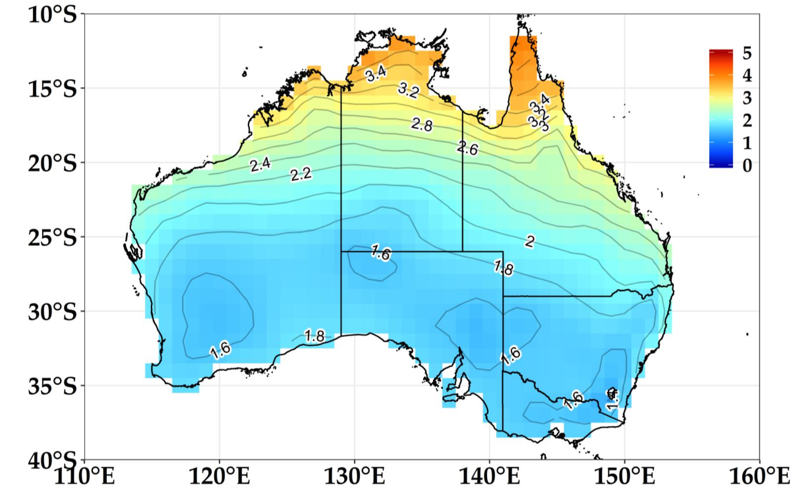
2015년 07월 - 2016년 12월에 대한 요약 통계량 (평균, 최대값, 최소값, 자료 개수) 및 평균 강수량 가시화

[활용 자료]

위성명 : NPP 기상위성
센서명 : CERES
자료 레벨 : SSF 1deg
자료 종류 : 날짜, 시간, 위도, 경도, 강수량, 지표면 특성, 운량
영역 : 호주
해상도 : 100 km
확장자 : NetCDF
기간 : 2015년 07월 15일 - 2016년 12월 21일

[자료 처리 방안 및 활용 분석 기법]

없음

[사용법]

입력 자료를 동일 디렉터리 위치
소스 코드를 실행 (Rscript Processing_Using_NetCDF_Format_of_NPP_CERES_SSF_1deg_Data.R)

가시화 결과 확인

[사용 OS]

Windows10

[사용 언어]

R v3.6.2
R Studio v1.2.5033

소스 코드

[명세]

메모리 해제

# Set Option
memory.limit(size = 9999999999999)

라이브러리 읽기

# Library Load
library(RNetCDF)
library(tidyverse)
library(metR)
library(colorRamps)
library(ggrepel)
library(extrafont)
library(sf)

파일 읽기

# File Read
sInputFileDirName = "INPUT_SSF1deg/*.nc"
sFileDirName = Sys.glob(sInputFileDirName)

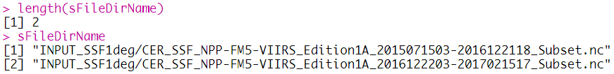
length(sFileDirName)
sFileDirName

NetCDF 파일 읽기

# NetCDF File Open
ncFile = open.nc(sFileDirName[iCount])

출력을 위한 파일명 초기화

# Set Output File Name
sFileDirNameSplit = unlist(str_split(string = sFileDirName[iCount], pattern = "_|/|\\."))
sOutputFileDirName = paste0('OUTPUT/', sFileDirNameSplit[5], "_", sFileDirNameSplit[7], ".OUT")

NetCDF 파일 읽기

# NetCDF File Read
ncData = read.nc(ncFile)

# print.nc(ncFile)
netcdf classic {
dimensions:
	time = UNLIMITED ; // (29240974 currently)
	The_8_most_prevalent_surface_types = 8 ;
	Conditions_clear__lower__upper__upper_over_lower = 4 ;
variables:
	NC_DOUBLE time(time) ;
		NC_CHAR time:long_name = "time" ;
		NC_CHAR time:units = "days since 1970-01-01 00:00:00" ;
		NC_DOUBLE time:_FillValue = 1.79769313486232e+308 ;
		NC_DOUBLE time:valid_range = 0, 39412.5 ;
	NC_FLOAT lon(time) ;
		NC_CHAR lon:long_name = "longitude" ;
		NC_CHAR lon:units = "degrees_east" ;
		NC_FLOAT lon:_FillValue = 3.40282346638529e+38 ;
		NC_FLOAT lon:valid_range = -180, 180 ;
	NC_FLOAT lat(time) ;
		NC_CHAR lat:long_name = "latitude" ;
		NC_CHAR lat:units = "degrees_north" ;
		NC_FLOAT lat:_FillValue = 3.40282346638529e+38 ;
		NC_FLOAT lat:valid_range = -90, 90 ;
	NC_DOUBLE Time_of_observation(time) ;
		NC_CHAR Time_of_observation:orig_name = "Time of observation" ;
		NC_CHAR Time_of_observation:units = "day" ;
		NC_CHAR Time_of_observation:format = "F18.9" ;
		NC_DOUBLE Time_of_observation:_FillValue = 1.79769313486232e+308 ;
		NC_DOUBLE Time_of_observation:valid_range = 2440000, 2480000 ;
	NC_FLOAT Longitude_of_CERES_FOV_at_surface(time) ;
		NC_CHAR Longitude_of_CERES_FOV_at_surface:orig_name = "Longitude of CERES FOV at surface" ;
		NC_CHAR Longitude_of_CERES_FOV_at_surface:units = "degrees" ;
		NC_CHAR Longitude_of_CERES_FOV_at_surface:format = "F18.9" ;
		NC_FLOAT Longitude_of_CERES_FOV_at_surface:_FillValue = 3.40282346638529e+38 ;
		NC_FLOAT Longitude_of_CERES_FOV_at_surface:valid_range = 0, 360 ;
	NC_FLOAT Colatitude_of_CERES_FOV_at_surface(time) ;
		NC_CHAR Colatitude_of_CERES_FOV_at_surface:orig_name = "Colatitude of CERES FOV at surface" ;
		NC_CHAR Colatitude_of_CERES_FOV_at_surface:units = "degrees" ;
		NC_CHAR Colatitude_of_CERES_FOV_at_surface:format = "F18.9" ;
		NC_FLOAT Colatitude_of_CERES_FOV_at_surface:_FillValue = 3.40282346638529e+38 ;
		NC_FLOAT Colatitude_of_CERES_FOV_at_surface:valid_range = 0, 180 ;
	NC_SHORT Surface_type_index(The_8_most_prevalent_surface_types, time) ;
		NC_CHAR Surface_type_index:orig_name = "Surface type index" ;
		NC_CHAR Surface_type_index:units = "N/A" ;
		NC_CHAR Surface_type_index:format = "I10" ;
		NC_SHORT Surface_type_index:_FillValue = 32767 ;
		NC_SHORT Surface_type_index:valid_range = 1, 20 ;
	NC_FLOAT Precipitable_water(time) ;
		NC_CHAR Precipitable_water:orig_name = "Precipitable water" ;
		NC_CHAR Precipitable_water:units = "centimeters" ;
		NC_CHAR Precipitable_water:format = "F18.9" ;
		NC_FLOAT Precipitable_water:_FillValue = 3.40282346638529e+38 ;
		NC_FLOAT Precipitable_water:valid_range = 0.00100000004749745, 10 ;
	NC_FLOAT Clear_layer_overlap_percent_coverages(Conditions_clear__lower__upper__upper_over_lower, time) ;
		NC_CHAR Clear_layer_overlap_percent_coverages:orig_name = "Clear/layer/overlap percent coverages" ;
		NC_CHAR Clear_layer_overlap_percent_coverages:units = "N/A" ;
		NC_CHAR Clear_layer_overlap_percent_coverages:format = "F18.9" ;
		NC_FLOAT Clear_layer_overlap_percent_coverages:_FillValue = 3.40282346638529e+38 ;
		NC_FLOAT Clear_layer_overlap_percent_coverages:valid_range = 0, 100 ;

// global attributes:
		NC_CHAR :Conventions = "CF-1.0" ;
		NC_CHAR :Subsetter_title = "ASDC CERES Subset" ;
		NC_CHAR :Subsetter_version = "2.9.b1" ;
		NC_CHAR :Subsetter_institution = "Atmospheric Science Data Center (ASDC) http://eosweb.larc.nasa.gov" ;
		NC_CHAR :Subsetter_history = "2017-12-29T02:00:57 -0500 SubsetCeresSsf" ;
		NC_CHAR :Subsetter_temporalFilter = "2015-07-15T00:00:00.000000Z to 2017-02-15T23:59:59.999999Z" ;
		NC_CHAR :Subsetter_spatialFilter = "POLYGON ((112.6593017578125 -44.285888671875, 112.6593017578125 -10.535888671875, 153.9678955078125 -10.535888671875, 153.9678955078125 -44.285888671875, 112.6593017578125 -44.285888671875))" ;
		NC_CHAR :Subsetter_parameterFilter = "none" ;
		NC_CHAR :platform = "NPP" ;
		NC_CHAR :history = "Fri Dec 29 02:17:45 2017: ncrcat -o CER_SSF_NPP-FM5-VIIRS_Edition1A_2015071503-2016122118_Subset.nc" ;
		NC_INT :nco_input_file_number = 4151 ;
		NC_CHAR :nco_input_file_list = "CER_SSF_NPP-FM5-VIIRS_Edition1A_100101.2015071503_Subset.nc

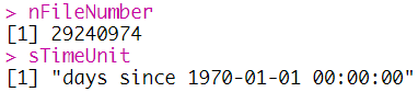
NetCDF 파일 갯수 및 Time 단위 가져오기

# Get Time Unit
nFileNumber = dim.inq.nc(ncFile, "time")$length
sTimeUnit = att.get.nc(ncFile, "time", "units")

NetCDF 변수 가져오기

# Get Variable
nDateTime = utcal.nc(sTimeUnit, ncData$time)
nLon  = ncData[["lon"]]
nLat  = ncData[["lat"]]
nTpw  = ncData[["Precipitable_water"]]
nSurfaceType = ncData[["Surface_type_index"]][1, ]
nClearFraction = ncData[["Clear_layer_overlap_percent_coverages"]][1, ]

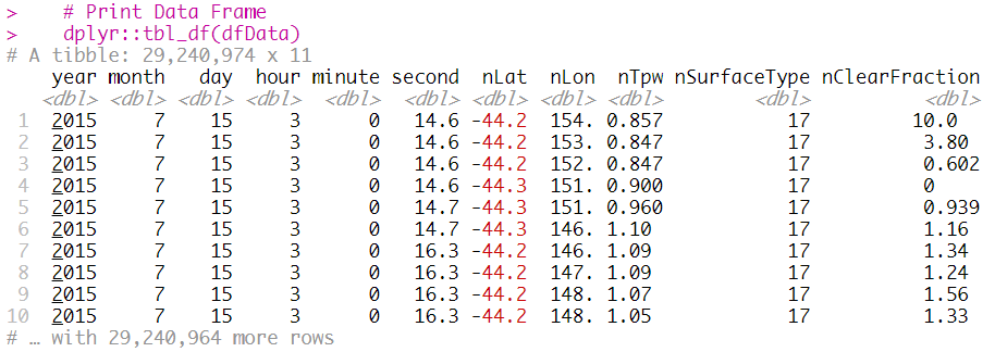
NetCDF 변수들을 Data Frame 형태로 초기화

# Set Data Frame
dfData = data.frame(nDateTime, nLat, nLon, nTpw, nSurfaceType, nClearFraction)
   
# Print Data Frame
dplyr::tbl_df(dfData)

Data Frame를 통해 L1 전처리
- 각 변수에 따라 최소값/최대값 설정

# L1 Processing Using Data Frame
dfDataL1 = dfData %>%
   dplyr::filter(
      between(nLat, -90.0, 90.0)
      , between(nLon, -180.0, 180.0)
      , between(nTpw, 0, 10)
      , between(nSurfaceType, 1, 20)
      , between(nClearFraction, 0, 100)
   )
   
# Print Data Frame
dplyr::tbl_df(dfDataL1)

L1 자료를 이용해서 L2 전처리
- NA 제거

# Delete NA Using L1 Data Frame
dfDataL2 = na.omit(dfData)

# Print Data Frame
dplyr::tbl_df(dfDataL2)

L2 자료를 출력
- 옵션 설명
  - sep : 구분자
  - file : 출력 파일명
  - append : 이어쓰기 여부
  - row.names : 행 이름 포함 여부
  - col.names : 열 이름 포함 여부

# Write Using L2 Data Frame
write.table(
   dfDataL2
   , sep = " "
   , file = sOutputFileDirName
   , append = FALSE
   , row.names = FALSE
   , col.names = FALSE
)

L2 자료를 이용해서 L3 전처리
- 공간 해상도 일치를 위해서 위/경도에 대한 정수 처리
- 해양 영역에 대한 마스킹 처리

# L3 Processing Using L2 Data Frame
dfDataL3 = dfDataL2 %>%
   dplyr::mutate(
      nRefLat = round(nLat, 0)
      , nRefLon = round(nLon, 0)
      , isLand = metR::MaskLand(dfDataL3$nRefLon, dfDataL3$nRefLat, mask = "world")
   ) %>%
   dplyr::filter(isLand == TRUE)

# Write Using L3 Data Frame
dplyr::glimpse(dfDataL3)

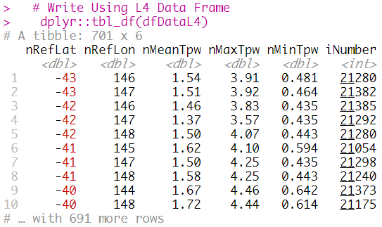
L3 자료를 이용해서 L4 전처리
- 2015년 07월 - 2016년 12월에 대한 가강수량의 요약 통계량 (평균, 최대값, 최소값, 개수)

# Mean For the Period 201507-201612 Using L3 Data Frame
dfDataL4 = dfDataL3 %>%
   dplyr::group_by(nRefLat, nRefLon) %>%
   dplyr::summarise(
      nMeanTpw = mean(nTpw, na.rm = TRUE)
      , nMaxTpw = max(nTpw, na.rm = TRUE)
      , nMinTpw = min(nTpw, na.rm = TRUE)
      , iNumber = n()
   )

# Write Using L4 Data Frame
dplyr::tbl_df(dfDataL4)

가시화를 위한 설정
- 폰트
- 컬러바
- 호주에 대한 Shape 지도

# Set Value for Visualization
font = "Palatino Linotype"
cbMatlab =  colorRamps::matlab.like(11)
mapAus = read_sf("INPUT/gadm36_AUS_shp/gadm36_AUS_1.shp")

L4 자료를 이용한 가시화
- 등고선
- 호주에 대한 Shape

# Visualization Using ggplot2
ggplot() +
   coord_fixed(ratio = 1.1) +
   theme_bw() +
   geom_tile(data = dfDataL4, aes(x = nRefLon, y = nRefLat, fill = nMeanTpw)) +
   geom_text_contour(data = dfDataL4, aes(x = nRefLon, y = nRefLat, z = nMeanTpw), stroke = 0.2) +
   geom_contour(data = dfDataL4, aes(x = nRefLon, y = nRefLat, z = nMeanTpw), color = "black", alpha = 0.3) +
   scale_fill_gradientn(colours = cbMatlab, limits=c(0, 5), breaks = seq(0, 5, 1), na.value = cbMatlab[length(cbMatlab)]) +
   theme(plot.title = element_text(face = "bold", size = 18, color = "black")) +
   theme(axis.title.x = element_text(face = "bold", size = 18, colour = "black")) +
   theme(axis.title.y = element_text(face = "bold", size=18, colour = "black", angle=90)) +
   theme(axis.text.x  = element_text(face = "bold", size=18, colour = "black")) +
   theme(axis.text.y  = element_text(face = "bold", size=18, colour = "black")) +
   metR::scale_x_longitude(expand = c(0, 0), breaks = seq(110, 160, 10), limits = c(110, 160)) +
   metR::scale_y_latitude(expand = c(0, 0), breaks = seq(-40, -10, 5), limits = c(-40, -10)) +
   geom_sf(data = mapAus, color = "black", fill = NA) +
   theme(legend.position = c(1, 1), legend.justification = c(1, 1)) +
   theme(legend.key=element_blank()) +
   theme(legend.text=element_text(size = 14, face = "bold")) +
   theme(legend.title=element_text(face = "bold", size = 14, colour = "black")) +
   labs(x = ""
        , y = ""
        , fill = ""
        , colour = ""
        , title  = ""
   ) +
   theme(legend.background=element_blank()) +
   theme(text=element_text(family = font)) +
   theme(plot.margin = unit(c(0, 8, 0, 0), "mm")) +
   ggsave(filename = paste0('FIG/Tpw.png'), width = 8, height = 10, dpi = 600)

[전체]

참고 문헌

[논문]

없음

[보고서]

없음

[URL]

없음

문의사항

[기상학/프로그래밍 언어]

sangho.lee.1990@gmail.com

[해양학/천문학/빅데이터]

saimang0804@gmail.com

저작자표시 동일조건 (새창열림)

'프로그래밍 언어 > R' 카테고리의 다른 글

[R] 고층/상층 기상 자료 (라디오존데)를 이용한 전처리 및 단열선도 (Skew T Log P) 가시화 (0)	2019.12.31
[R] 새해 경자년에 해돋이/일출/해 뜨는 시간 가시화 (0)	2019.12.31
[R] NetCDF 형식인 NPP/CERES SSF 기상위성 자료를 이용하여 아스키 (ASCII) 형식으로 처리 (0)	2019.12.28
[R] 다수의 날짜정보를 컬럼으로 가진 DataFrame 에서의 컬럼 제어 방법 (0)	2019.12.21
[R] 동아시아 대기질 이미지 영상을 통해 크롤링 및 애니메이션 구현 (0)	2019.12.08

정보

내용

[특징]

[기능]

[활용 자료]

[자료 처리 방안 및 활용 분석 기법]

[사용법]

[사용 OS]

[사용 언어]

소스 코드

[명세]

[전체]

참고 문헌

[논문]

[보고서]

[URL]

문의사항

'프로그래밍 언어 > R' 카테고리의 다른 글

티스토리툴바