[IDL] 아이디엘 HDF 형식인 Terra/MODIS 극궤도 기상 위성 자료를 이용한 총 오존량 가시화

 정보

• 업무명    : 아이디엘 HDF 형식인 Terra/MODIS 극궤도 기상 위성 자료를 이용한 총 오존량 가시화

• 작성자    : 이상호

• 작성일    : 2019-08-29

• 설   명    :

• 수정이력 :

  • 2020-03-24 : 소스 코드 명세 추가

 

 내용

[개요]

• 안녕하세요? 기상 연구 및 웹 개발을 담당하고 있는 해솔입니다.

• TOMS (Total Ozone Mapping Spectrometer)는 1978 년 11 월 NIMBUS 위성 7호에서 처음 시작하여 매일 총 오존량의 전 세계 분포를 측정했습니다.

• 이러한 TOMS는 1993년 05월 06일까지 약 14.5 년 동안 계속 관측하였으며 남극의 봄 기간에 심한 오존층 파괴로 인한 오존 구멍이 발견되었을 때 TOMS의 이름이 널리 알려졌습니다.

• TOMS 데이터는 남극 대륙의 오존 구멍 면적의 범위뿐만 아니라 80년대 초 이후의 시간에 따른 오존 구멍의 발달을 분명히 보여주었습니다.

• 그 밖에 Meteor 위성 3호, ADEOS 위성들도 우주에서 총 오존 관측을 수행했으며 최근에 많은 극궤도 기상위성들이 오존층 모니터링을 하고 있습니다.

• 오늘 포스팅에서는 HDF 형식인 Terra/MODIS 극궤도 기상 위성 자료를 이용한 총 오존량 가시화를 소개해 드리고자 합니다.

 

[특징]

• HDF 기상 위성 자료를 이용하여 정성적으로 가시화하기 위한 도구가 필요하며 이 프로그램은 이러한 목적을 달성하기 위해 고안된 소프트웨어

 

[기능]

• Terra/MODIS 극궤도 기상 위성 자료에 대한 위경도 및 총 오존량 읽기

• 위경도 및 총 오존량에 대한 통계 수치 (최대값, 최소값, 평균) 확인

• 지상 관측소의 위/경도를 이용하여 맵핑

• 도법 (cylindrical, satellite)에 따라 가시화 및 컬러바 설정

• 이미지 저장

 

[사용법]

• 입력 자료를 동일 디렉터리에 위치

• 소스 코드를 실행 (idl -e Visualization_Using_Terra_MODIS_Data)

• 가시화 결과를 확인

 

[사용 OS]

• Linux

• Windows 10

 

[사용 언어]

• IDL v8.5

 

 소스 코드

• 해당 작업을 하기 위한 컴파일 및 실행 코드는 IDL로 작성되었으며 가시화를 위한 라이브러리는 Coyote's Guide to IDL Programming를 이용하였습니다.
  

• 소스 코드는 단계별로 수행하며 상세 설명은 다음과 같습니다.
  

  • 1 단계는 주 프로그램은 작업 경로 설정, HDF 파일 읽기, 변수 전처리하여 메모리상에 저장하고 가시화를 위한 초기 설정합니다.
    

  • 2 단계는 plot 또는 contour 매핑에 따라 영상 장면 표출하여 이미지 형식으로 저장합니다. 이 과정에서 포스트 스크립트 (PS) 형식에서 PNG로 변환합니다.

 

[명세]

• 작업 환경 설정

cd, 'D:\할 일\Program\각종 자료\Aerosol mapping+RGB\modis hdf_ps_RGB x\Ozone'

 

• 파일 찾기

hdf_files=file_search('./INPUT/MOD07_L2*.hdf',count=count)

 

• HDF 파일 읽기

  • 반복문 수행하면서 hdf_files 및 hdf_sd_start 파일 읽기

for k=0,count-1, 1 do begin

	hdf_file=hdf_files(k)
  	print, hdf_file

  	sd_id=hdf_sd_start(hdf_file, /read)

  	# 생략

endfor

 

• 각 변수에 대한 전처리

  • hdf_sd_nametoindex 및 hdf_sd_getdata를 통해 위도 (lat), 경도 (lon), 총 오존량 (var) 디지털값 설정

  • hdf_sd_attrfind를 통해 결측값 (_FillValue), 유효 범위 (valid_range), scale_factor, add_offset 변수 설정

  • where를 통해 결측값 및 유효범위에 제외한 후 scale_factor 및 add_offset를 통해 디지털값을 물리적 변수로 변환

sds_index = hdf_sd_nametoindex(sd_id, 'Latitude')
    sds_id = hdf_sd_select(sd_id, sds_index)
    sds_id_fill = hdf_sd_attrfind(sds_id, '_FillValue')
    hdf_sd_attrinfo, sds_id, sds_id_fill, data=fill
    sds_id_valid = hdf_sd_attrfind(sds_id, 'valid_range')
    hdf_sd_attrinfo, sds_id, sds_id_valid, data=valid
    sds_id_scale = hdf_sd_attrfind(sds_id, 'scale_factor')
    hdf_sd_attrinfo, sds_id, sds_id_scale, data=scale
    sds_id_add = hdf_sd_attrfind(sds_id, 'add_offset')
    hdf_sd_attrinfo, sds_id, sds_id_add, data=offset
    hdf_sd_getdata, sds_id, data
    data=float(data)
    loc1 = where( ((data lt valid[0]) or (data gt valid[1]) or (data eq fill[0])), nloc1, complement=loc2, ncomplement=nloc2 )
    if (nloc1 gt 0) then data[loc1] = !values.f_nan
    if (nloc2 gt 0) then data[loc2] = scale[0]*(data[loc2]-offset[0])
lat = data


sds_index = hdf_sd_nametoindex(sd_id, 'Longitude')
    sds_id = hdf_sd_select(sd_id, sds_index)
    sds_id_fill = hdf_sd_attrfind(sds_id, '_FillValue')
    hdf_sd_attrinfo, sds_id, sds_id_fill, data=fill
    sds_id_valid = hdf_sd_attrfind(sds_id, 'valid_range')
    hdf_sd_attrinfo, sds_id, sds_id_valid, data=valid
    sds_id_scale = hdf_sd_attrfind(sds_id, 'scale_factor')
    hdf_sd_attrinfo, sds_id, sds_id_scale, data=scale
    sds_id_add = hdf_sd_attrfind(sds_id, 'add_offset')
    hdf_sd_attrinfo, sds_id, sds_id_add, data=offset
    hdf_sd_getdata, sds_id, data
    data = float(data)
    loc1 = where( ((data lt valid[0]) or (data gt valid[1]) or (data eq fill[0])), nloc1, complement=loc2, ncomplement=nloc2 )
    if (nloc1 gt 0) then data[loc1] = !values.f_nan
    if (nloc2 gt 0) then data[loc2] = scale[0]*(data[loc2]-offset[0]) 
lon = data

sds_index = hdf_sd_nametoindex(sd_id, 'Total_Ozone')
    sds_id = hdf_sd_select(sd_id, sds_index)
    sds_id_fill = hdf_sd_attrfind(sds_id, '_FillValue')
    hdf_sd_attrinfo, sds_id, sds_id_fill, data=fill
    sds_id_valid = hdf_sd_attrfind(sds_id, 'valid_range')
    hdf_sd_attrinfo, sds_id, sds_id_valid, data=valid
    sds_id_scale = hdf_sd_attrfind(sds_id, 'scale_factor')
    hdf_sd_attrinfo, sds_id, sds_id_scale, data=scale
    sds_id_add = hdf_sd_attrfind(sds_id, 'add_offset')
    hdf_sd_attrinfo, sds_id, sds_id_add, data=offset
    hdf_sd_getdata, sds_id, data
    data=float(data)
    loc1 = where( ((data lt valid[0]) or (data gt valid[1]) or (data eq fill[0])), nloc1, complement=loc2, ncomplement=nloc2 )
    if (nloc1 gt 0) then data[loc1] = !values.f_nan
    if (nloc2 gt 0) then data[loc2] = scale[0]*(data[loc2]-offset[0])
var = data

hdf_sd_endaccess, sds_id
hdf_sd_end, sd_id

 

• 위/경도 및 오존량에 대한 통계 수치 확인

  • 최소값 : min

  • 평균 : mean

  • 최대값 : max

;============================
;     Statistical analysis
;============================
print, min(lon, /nan), mean(lon, /nan), max(lon, /nan)
print, min(lat, /nan), mean(lat, /nan), max(lat, /nan)
print, min(var, /nan), mean(var, /nan), max(var, /nan)

 

• 기타 설정

  • 표출 영역 (latmin, lonmin, latmax, lonmax) 설정

  • 지상 관측소의 위도 (point_lat), 경도 (point_lon), 지점명 (point_name) 설정

;==================================
;   Option
;==================================
start_color=0  &  end_color=255  &  colorn=end_color-start_color+1

latmin=-90  &  lonmin=0  &  latmax=90  &  lonmax=360   ; satellite

point_lon = [126.14, 126.16, 126.93]
point_lat = [37.23,  33.29,  37.56]
point_name = ['a', 'b', 'c']

 

• 가시화를 위한 초기 설정

  • set_plot를 통해 포스트 스크립트 (Post Script, PS) 형식으로 저장 및 세부 옵션

    • 그림 저장명 : filename

    • 폰트 : /SCHOOLBOOK

    • 폰트 굵게 : /BOLD

  • usersym를 통해 매핑을 위한 심볼 설정

  • 중심 위도 (clat), 중심 경도 (clon) 설정

  • cgmap_set를 통해 도법 (satellite) 설정

n_color = 256

ps_name = file_basename(hdf_file, '.hdf')  ; file name  Change
print, ps_name

set_plot,'ps'
device, filename=ps_name+'.ps', decomposed=0, bits=8, /color, xsize=13, ysize=12, /inches, $
/SCHOOLBOOK, /BOLD

!p.font=0  &  !p.charsize=2.0  &  !p.charthick=1.6  &  !p.multi=[0,1,1]
usersym, [0.1,0.1,-0.1,-0.1,0.1], [-0.1,0.1,0.1,-0.1,-0.1], /fill

clat = 0.0  & clon = 128.2
cgmap_set, /satellite, sat_p=[42159.934825,0,0], clat, clon, charsize=1.0, limit=[-90,-180,90,180], $
position=[0.10,0.15,0.9,0.95], /isotropic, color='white'

zmin = 300. & zmax = 500.     
cgloadct, 33, bottom=0, ncolor=n_color

 

• 매핑을 위한 설정 및 가시화 (1) : points

  • 총 오존량의 최대/최소값 : zmin 및 zmax

  • cgloadct를 통해 컬러바 설정

  • 위/경도 개수 (dims)만큼 반복문을 수행하면서 분기문 수행

    • 총 오존량 > 0 이상인 경우

    • 최대/최소 위/경도인 경우

  • plots를 통해 위/경도에 따른 총 오존량 컬러 (color) 가시화

;===========================
;     Mapping : plot
;===========================  
zmin = 300.  &  zmax = 500.     
cgloadct, 33, bottom=0, ncolor=n_color
tvlct, r, g, b, /Get

latmin=32 & lonmin=120 & latmax=42 & lonmax=132 

for i=0L, dims[0]-1 do begin
for j=0L, dims[1]-1 do begin

  val=var[i,j]
  
  if(val gt 0 ) then begin
  if( (lat[i,j] gt latmin) and (lat[i,j] lt latmax) ) then begin
  if( (lon[i,j] gt lonmin) and (lon[i,j] lt lonmax) ) then begin
  	plots, lon[i,j], lat[i,j], psym=8, symsize=2.5, color=start_color+colorn*(val-zmin)/(zmax-zmin)
  endif
  endif
  endif
endfor
endfor

 

• 매핑을 위한 설정 및 가시화 (2) : contour

  • 총 오존량의 최대/최소값 : zmin 및 zmax

  • cgloadct를 통해 컬러바 설정

  • cgcontour를 통해 총 오존량 등고선 가시화

;========================================
;     Mapping : Contour fill, contour 
;========================================
zmin = 300.  &   zmax = 500.  

levels=255
step=(zmax-zmin)/levels
userlevels=findgen(levels)*step + zmin
cgloadct, 33, ncolors=levels, bottom=0
cgcontour, var, lon, lat, /overplot, /cell_fill, nlevels=levels,  $
	C_THICK=3, C_CHARSIZE=2, C_CHARTHICK=2, c_color=indgen(levels), levels=userlevels

 

• 도법에 대한 격자 보조선 설정

  • cgmap_grid를 기준 위/경도 (lats, lons)에 따라 텍스트 (lats_names, lons_names) 및 격자 보조선 삽입

  • cgtext를 통해 그림 제목 삽입

lats = [-90, -60, -30, 0, 30, 60, 90]
lats_names = ['',textoidl('60\circS', font=0), textoidl('30\circS', font=0), ' ', textoidl('30\circN', font=0),textoidl('60\circN', font=0), '']
lons = [10, 70, 100, 130, 160, -170, -10]
lons_names = ['',textoidl('70\circE'), textoidl('100\circE'), textoidl('130\circE'), textoidl('160\circE'), textoidl('170\circW'),'']

cgmap_grid, color='black', /label, lats=lats,  latlabel=160, lonlabel=-5, latnames=lats_names, lons=lons, lonnames=lons_names,  $
clip_text=0, linestyle=1, noclip=0, /horizon, charsize=1.7                  

cgtext, 0.5, 0.965, ps_name, charsize=2, charthick=1.2, alignment=0.5, color='black', font=0, /normal ; GOCI(1)

 

• 포스트 스크립트 형식 (PS)을 PNG로 변환

  • device를 통해 포스크 스크립트 정상 종료

  • convert를 통해 PNG 이미지 형태로 변환

device, /close_file

com  = 'convert -flatten -background white '+ps_name+'.ps'+' '+'OUTPUT/'+file_basename(ps_name, '.ps')+'.png'
spawn, com

file_delete, ps_name+'.ps'

 

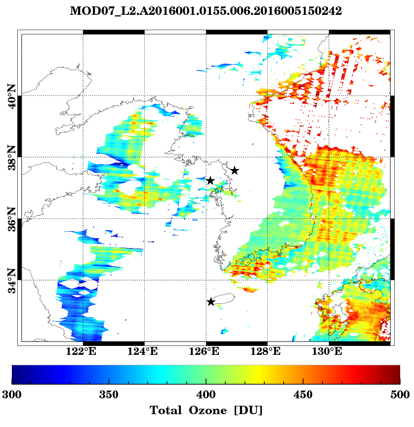
• MODIS 자료를 이용하여 한반도 총 오존량 분포

 

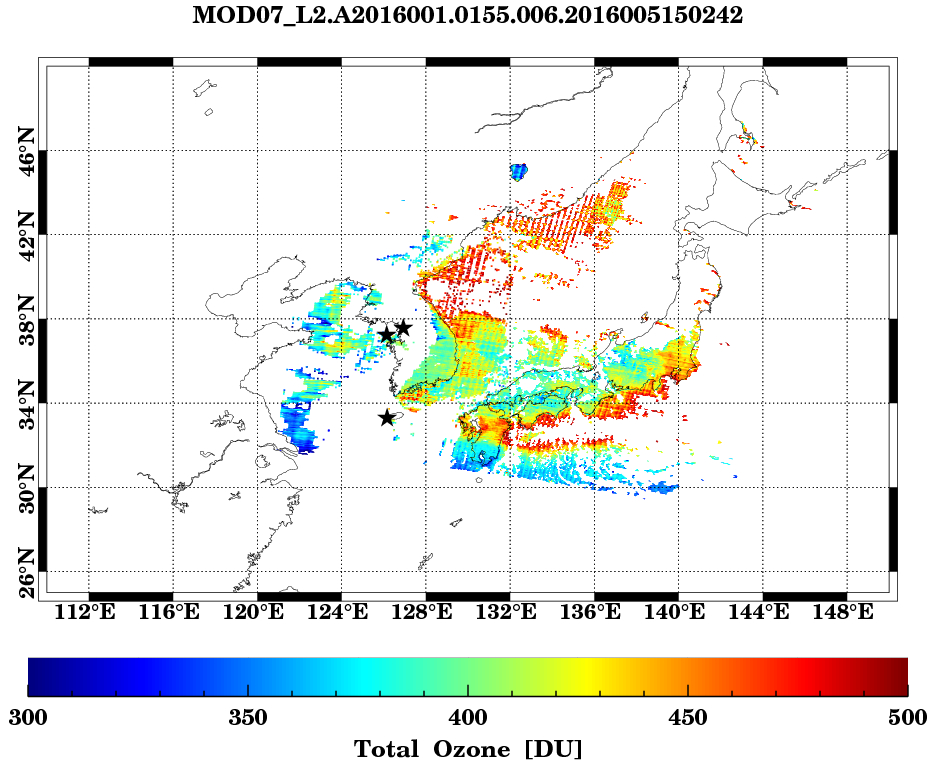
• MODIS 자료를 이용하여 동아시아 총 오존량 분포

 

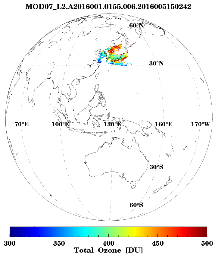
• MODIS 자료를 이용하여 전구 총 오존량 분포

 

[전체] 

	pro Visualization_Using_Terra_MODIS_Data
	cd, 'D:\할 일\Program\각종 자료\Aerosol mapping+RGB\modis hdf_ps_RGB x\Ozone'
	;===================================
	; hdf read
	;===================================
	hdf_files=file_search('./INPUT/MOD07_L2*.hdf',count=count)
	for k=0,count-1, 1 do begin
	hdf_file=hdf_files(k)
	print, hdf_file
	sd_id=hdf_sd_start(hdf_file, /read)
	sds_index = hdf_sd_nametoindex(sd_id, 'Latitude')
	sds_id = hdf_sd_select(sd_id, sds_index)
	sds_id_fill = hdf_sd_attrfind(sds_id, '_FillValue')
	hdf_sd_attrinfo, sds_id, sds_id_fill, data=fill
	sds_id_valid = hdf_sd_attrfind(sds_id, 'valid_range')
	hdf_sd_attrinfo, sds_id, sds_id_valid, data=valid
	sds_id_scale = hdf_sd_attrfind(sds_id, 'scale_factor')
	hdf_sd_attrinfo, sds_id, sds_id_scale, data=scale
	sds_id_add = hdf_sd_attrfind(sds_id, 'add_offset')
	hdf_sd_attrinfo, sds_id, sds_id_add, data=offset
	hdf_sd_getdata, sds_id, data
	data=float(data)
	loc1 = where( ((data lt valid[0]) or (data gt valid[1]) or (data eq fill[0])), nloc1, complement=loc2, ncomplement=nloc2 )
	if (nloc1 gt 0) then data[loc1] = !values.f_nan
	if (nloc2 gt 0) then data[loc2] = scale[0]*(data[loc2]-offset[0])
	lat = data
	sds_index = hdf_sd_nametoindex(sd_id, 'Longitude')
	sds_id = hdf_sd_select(sd_id, sds_index)
	sds_id_fill = hdf_sd_attrfind(sds_id, '_FillValue')
	hdf_sd_attrinfo, sds_id, sds_id_fill, data=fill
	sds_id_valid = hdf_sd_attrfind(sds_id, 'valid_range')
	hdf_sd_attrinfo, sds_id, sds_id_valid, data=valid
	sds_id_scale = hdf_sd_attrfind(sds_id, 'scale_factor')
	hdf_sd_attrinfo, sds_id, sds_id_scale, data=scale
	sds_id_add = hdf_sd_attrfind(sds_id, 'add_offset')
	hdf_sd_attrinfo, sds_id, sds_id_add, data=offset
	hdf_sd_getdata, sds_id, data
	data = float(data)
	loc1 = where( ((data lt valid[0]) or (data gt valid[1]) or (data eq fill[0])), nloc1, complement=loc2, ncomplement=nloc2 )
	if (nloc1 gt 0) then data[loc1] = !values.f_nan
	if (nloc2 gt 0) then data[loc2] = scale[0]*(data[loc2]-offset[0])
	lon = data
	sds_index = hdf_sd_nametoindex(sd_id, 'Total_Ozone')
	sds_id = hdf_sd_select(sd_id, sds_index)
	sds_id_fill = hdf_sd_attrfind(sds_id, '_FillValue')
	hdf_sd_attrinfo, sds_id, sds_id_fill, data=fill
	sds_id_valid = hdf_sd_attrfind(sds_id, 'valid_range')
	hdf_sd_attrinfo, sds_id, sds_id_valid, data=valid
	sds_id_scale = hdf_sd_attrfind(sds_id, 'scale_factor')
	hdf_sd_attrinfo, sds_id, sds_id_scale, data=scale
	sds_id_add = hdf_sd_attrfind(sds_id, 'add_offset')
	hdf_sd_attrinfo, sds_id, sds_id_add, data=offset
	hdf_sd_getdata, sds_id, data
	data=float(data)
	loc1 = where( ((data lt valid[0]) or (data gt valid[1]) or (data eq fill[0])), nloc1, complement=loc2, ncomplement=nloc2 )
	if (nloc1 gt 0) then data[loc1] = !values.f_nan
	if (nloc2 gt 0) then data[loc2] = scale[0]*(data[loc2]-offset[0])
	var = data
	hdf_sd_endaccess, sds_id
	hdf_sd_end, sd_id
	dims = size(var, /dimensions)
	; print, dims[0], dims[1]
	;============================
	; Statistical analysis
	;============================
	print, min(lon, /nan), mean(lon, /nan), max(lon, /nan)
	print, min(lat, /nan), mean(lat, /nan), max(lat, /nan)
	print, min(var, /nan), mean(var, /nan), max(var, /nan)
	;==================================
	; Option
	;==================================
	start_color=0 & end_color=255 & colorn=end_color-start_color+1
	; latmin=min(lat, /nan) & lonmin=min(lon, /nan) & latmax=max(lat, /nan) & lonmax= max(lon, /nan)
	latmin=-90 & lonmin=0 & latmax=90 & lonmax=360 ; satellite
	; latmin=32 & lonmin=120 & latmax=42 & lonmax=132 ; GOCI (1), Hanbando
	; latmin=25 & lonmin=110 & latmax=50 & lonmax=150 ; GOCI (2), East asia
	point_lon = [126.14, 126.16, 126.93]
	point_lat = [37.23, 33.29, 37.56]
	point_name = ['a', 'b', 'c']
	;===============================================
	; dist
	;===============================================
	; for i=0L, 2 do begin
	;
	; loc1 = where(finite(var) eq 1, nloc1)
	; if (nloc1 gt 0) then distance = sqrt( ((lon[loc1]-point_lon[i])^2) + ((lat[loc1]-point_lat[i])^2) )
	;
	; loc1 = where( (distance eq min(distance, /nan)) and (finite(var) eq 1) , nloc1 )
	; print, var[loc1]
	; ;R[i] = var[loc1]
	;
	; print, loc1, point_lon[i]-lat[loc1], point_lon[i]-lon[loc1], var[loc1], r[i]
	; endfor
	;
	;===============================================
	; cylindrical plot
	;===============================================
	; n_color = 10
	n_color = 256
	clat = 0.0 & clon = (lonmin+lonmax)/2.0
	ps_name = file_basename(hdf_file, '.hdf') ; file name Change
	print, ps_name
	set_plot,'ps'
	device, filename=ps_name+'.ps', decomposed=0, bits=8, /color, xsize=13, ysize=12, /inches, $
	/SCHOOLBOOK, /BOLD
	; /PALATINO, /BOLD
	; /helvetica, /bold
	; /TIMES, /BOLD
	!p.font=0 & !p.charsize=2.0 & !p.charthick=1.6 & !p.multi=[0,1,1]
	usersym, [0.1,0.1,-0.1,-0.1,0.1], [-0.1,0.1,0.1,-0.1,-0.1], /fill
	; usersym, 17.2*[0,1,1,0,0]/9, 3.9*[0,0,1,1,0]/2, /fill
	; plotsym, 8, 0.5, /fill
	; cgmap_set, /cylindrical ,clat , clon, charsize=1.0, limit=[latmin,lonmin,latmax,lonmax], $
	; position=[0.10, 0.15, 0.9, 0.95], /isotropic , /noborder, color=0 ; satellite
	;; position=[0.05, 0.2, 0.95, 0.92], /isotropic , /noborder, color=0 ; GOCI (1)
	;; position=[0.05, 0.1, 0.95, 0.95], /isotropic , /noborder, color=0 ; GOCI (2)
	clat = 0.0 & clon = 128.2
	cgmap_set, /satellite, sat_p=[42159.934825,0,0], clat, clon, charsize=1.0, limit=[-90,-180,90,180], $
	position=[0.10,0.15,0.9,0.95], /isotropic, color='white'
	;===========================
	; Scene line
	;===========================
	; loadct, 0
	; tvlct, r, g, b, /Get
	; for i=0L, (dims[0]*dims[1])-1 do begin
	; val=var[i]
	; if ( (lat[i] ge latmin) and (lat[i] le latmax) ) then begin
	; if ( (lon[i] ge lonmin) and (lon[i] le lonmax) ) then begin
	; plots, lon[i], lat[i], psym=8, symsize=1, color=235
	; endif
	; endif
	; endfor
	;===========================
	; Mapping : plot
	;===========================
	zmin = 300. & zmax = 500.
	cgloadct, 33, bottom=0, ncolor=n_color
	tvlct, r, g, b, /Get
	latmin=32 & lonmin=120 & latmax=42 & lonmax=132
	for i=0L, dims[0]-1 do begin
	for j=0L, dims[1]-1 do begin
	val=var[i,j]
	if(val gt 0 ) then begin
	if( (lat[i,j] gt latmin) and (lat[i,j] lt latmax) ) then begin
	if( (lon[i,j] gt lonmin) and (lon[i,j] lt lonmax) ) then begin
	plots, lon[i,j], lat[i,j], psym=8, symsize=2.5, color=start_color+colorn*(val-zmin)/(zmax-zmin)
	endif
	endif
	endif
	endfor
	endfor
	;========================================
	; Mapping : Contour fill, contour
	;========================================
	zmin = 300. & zmax = 500.
	levels=255
	step=(zmax-zmin)/levels
	userlevels=findgen(levels)*step + zmin
	cgloadct, 33, ncolors=levels, bottom=0
	cgcontour, var, lon, lat, /overplot, /cell_fill, nlevels=levels, $
	C_THICK=3, C_CHARSIZE=2, C_CHARTHICK=2, c_color=indgen(levels), levels=userlevels
	; loadct, 0
	; levels = 8
	; step = (zmax - zmin) / levels
	; userlevels = fIndgen(levels)*step + zmin
	; cgcontour, var, lon, lat, /OVERPLOT, nlevels=levels, $
	; C_LABELS=userlevels, C_CHARSIZE=5, C_CHARTHICK=2, $
	; color=0
	;==========================
	; point
	;===========================
	; loadct, 0
	; plotsym, 3, 1, /fill
	; plots,point_lon,point_lat,PSYM=8, symsize=2, color=0
	;
	; cgloadct, 33, bottom=0, ncolor=n_color
	;=====================================
	; Colorbar (vertical, horizon)
	;=====================================
	; cgcolorbar,range=[zmin,zmax], bottom=0, ncolor=n_color, position=[0.15,0.935,0.85,0.97], $
	; /vertical, charsize=1.8, /right, /fit, ytickinterval=50, yminor=5, $
	; xtickinterval=0, xminor=0, xstyle=1, ystyle=1, xthick=5, ythick=5, ticklen=0.299
	; GOCI (1)
	; cgcolorbar, range=[zmin,zmax], bottom=0, ncolor=n_color, position=[0.1,0.08,0.145,0.92], $
	; yminor=0, ytickinterval=0, xminor=5, xstyle=1+8, ystyle=4, $
	; xthick=5, ythick=5, ticklen=0.29999, charsize=1.9
	; GOCI (2)
	; cgcolorbar, range=[zmin,zmax], bottom=0, ncolor=n_color, position=[0.1,0.03,0.145,0.97], $
	; yminor=0, ytickinterval=0, xminor=5, xstyle=1+8, ystyle=4, $
	; xthick=5, ythick=5, ticklen=0.29999, charsize=1.9
	;
	; satellite
	cgcolorbar, range=[zmin,zmax], bottom=0, ncolor=n_color, position=[0.15,0.09,0.85,0.13], $
	yminor=0, ytickinterval=0, xminor=5, xstyle=1+8, ystyle=4, $
	xthick=5, ythick=5, ticklen=0.29999, charsize=1.9
	cgtext, 0.5, 0.03, 'Total Ozone [DU]', charsize=2, charthick=1.2, alignment=0.5, color='black', font=0, /normal
	;=====================================
	; Map draw
	;=====================================
	cgmap_gshhs, 'gshhg'+path_sep()+'gshhs_i.b', color='black', /outline, level=4, thick=1.0
	; cgmap_continents, /continents, /hires, color='black', mlinethick=0.001, thick=1.0, limit=[-90,-180,90,180]
	;=====================================
	; Map grid draw
	;=====================================
	; lats = [-90:90:2] ; GOCI (1)
	; lons = [-360:180:2] ; GOCI (1)
	;; lats = [-90:90:4] ; GOCI (2)
	;; lons = [-360:180:4] ; GOCI (2)
	;
	; lats_names = textoidl(string(lats)+'\circN ')
	; lons_names = textoidl(string(lons)+'\circE ')
	;
	; cgmap_grid, color='black', charsize=1.8, thick=2.5, lats=lats, latnames=lats_names, lons=lons, lonnames=lons_names, $
	; linestyle=1, label=1, bthick=300, /box_axes, blabel=1, latdel=4, londel=4
	; satellite
	lats = [-90, -60, -30, 0, 30, 60, 90]
	lats_names = ['',textoidl('60\circS', font=0), textoidl('30\circS', font=0), ' ', textoidl('30\circN', font=0),textoidl('60\circN', font=0), '']
	lons = [10, 70, 100, 130, 160, -170, -10]
	lons_names = ['',textoidl('70\circE'), textoidl('100\circE'), textoidl('130\circE'), textoidl('160\circE'), textoidl('170\circW'),'']
	cgmap_grid, color='black', /label, lats=lats, latlabel=160, lonlabel=-5, latnames=lats_names, lons=lons, lonnames=lons_names, $
	clip_text=0, linestyle=1, noclip=0, /horizon, charsize=1.7
	cgtext, 0.5, 0.965, ps_name, charsize=2, charthick=1.2, alignment=0.5, color='black', font=0, /normal ; GOCI(1)
	; cgtext, 0.5, 0.88, ps_name, charsize=2, charthick=1.2, alignment=0.5, color='black', font=0, /normal ; GOCI(2)
	device, /close_file
	com = 'convert -flatten -background white '+ps_name+'.ps'+' '+'OUTPUT/'+file_basename(ps_name, '.ps')+'.png'
	spawn, com
	file_delete, ps_name+'.ps'
	endfor
	end

view raw Visualization_Using_Terra_MODIS_Data.pro hosted with ❤ by GitHub

 

 참고 문헌

[논문]

• 없음

[보고서]

• 없음

[URL]

• 없음

 

 문의사항

[기상학/프로그래밍 언어]

• sangho.lee.1990@gmail.com

[해양학/천문학/빅데이터]

• saimang0804@gmail.com