

정보
- 업무명 : WRF 모델 자료로부터 기상 변수 추출 및 단열선도 시각화 그리고 RadioSonde 패키지 내 단열선도 X축 커스터마이징 (켈빈 to 섭씨)
- 작성자 : 박진만
- 작성일 : 2021-01-18
- 설 명 :
- 수정이력 :
내용
[개요]
- 안녕하세요? 기상 연구 및 웹 개발을 담당하고 있는 해솔입니다.
- 이번 포스팅에서는 R의 패키지 중 하나인 RadioSonde 패키지를 소개하고자 합니다.
- 해당 패키지의 경우 손쉽게 Skew-T log-p 단열선도를 시각화 할 수 있지만 x축이 화씨 온도로만 표현이 가능합니다.
- 따라서 이를 섭씨 온도로 바꾸는 방법을 설명하고자 합니다.
[특징]
- 오픈소스 라이브러리 커스터마이징
[기능]
- 단열선도의 화씨 온도를 섭씨 온도로 변환하기
[활용 자료]
- 소스코드 참조
[자료 처리 방안 및 활용 분석 기법]
- 없음
[사용법]
- 실행방법 참조
[사용 OS]
- Windows 10
[사용 언어]
- R v4.0.3
소스 코드
[명세]
- 필수 입력자료
profile.csv
0.00MB
20230802_YARDSTICK.zip
0.45MB
- 라이브러리 및 커스터마이징된 서브 함수 읽기
library(RadioSonde)
library(data.table)
library(tidyverse)
library(lubridate)
library(dplyr)
library(RNetCDF)
library(weathermetrics)

source("./sub_pro_sonde.R")
- 서브함수는 아래와 같은 코드로 커스터마이징
- 커스터마이징된 소스코드는 하단에서 다운로드 받을 수 있음
plot_sonde <- function (dataframe, skewT=TRUE, winds=FALSE, site = "", title = "",
            windplot = NULL, s = 3., col = c(1, 2), ... ){
    #
    # Copyright 2001,2002 Tim Hoar, Eric Gilleland, and Doug Nychka
    #
    # This file is part of the RadioSonde library for R and related languages.
    #
    # RadioSonde is free software; you can redistribute it and/or modify
    # it under the terms of the GNU General Public License as published by
    # the Free Software Foundation; either version 2 of the License, or
    # (at your option) any later version.
    #
    # RadioSonde is distributed in the hope that it will be useful,
    # but WITHOUT ANY WARRANTY; without even the implied warranty of
    # MERCHANTABILITY or FITNESS FOR A PARTICULAR PURPOSE.  See the
    # GNU General Public License for more details.
    #
    # You should have received a copy of the GNU General Public License
    # along with RadioSonde; if not, write to the Free Software
    # Foundation, Inc., 59 Temple Place, Suite 330, Boston, MA  02111-1307  USA
    #

    msg <- deparse(match.call())

    if( skewT & winds){

      #
      # Plot the SKEW-T, log p diagram and the wind profile.
      #

      # Need some room for both the skewT plot and the wind profile.

      mar.skewt <- c(5.0999999999999996, 1.1000000000000001,
                     2.1000000000000001, 5.0999999999999996)
      skewt.plt <- skewt.axis1(mar = mar.skewt)$plt
      title(title)

      if(is.null(windplot)) {
        windplot <- skewt.plt
        windplot[1] <- 0.8
        windplot[2] <- 0.95

      } else if( (windplot[2] < windplot[1]) |
                 (windplot[4] < windplot[3]) ) {
        stop("plot region (windplot) too small to add second plot")
      }

      first.par <- par()

      # Draw the SKEW-T, log p diagram
      # Draw background and overlay profiles

      skewt.axis1()
      skewt.lines1(dataframe$temp,  dataframe$press, col = col[1], ...)
      skewt.lines1(dataframe$dewpt, dataframe$press, col = col[2], ...)

      #
      # Draw the windplot in the "space allocated"
      # top and bottom mar the same as skewt
      #
      print( windplot)
      par(new = TRUE, pty = "m", plt = windplot, err = -1.)
      plotwind(dataframe = dataframe, size = s, legend = FALSE)
      par(plt = first.par$plt, mar = first.par$mar, new = FALSE, pty = first.par$
            pty, usr = first.par$usr)
      #       title1 <- paste(site, ": ", month.year, " ", time, sep = "")
      invisible()

    } else if( skewT & !winds) {

      #
      # Draw the SKEW-T, log p diagram
      # Draw background and overlay profiles
      #

      skewt.axis1()
      skewt.lines1(dataframe$temp,  dataframe$press, col = col[1], ...)
      skewt.lines1(dataframe$dewpt, dataframe$press, col = col[2], ...)
      title(title)

    } else if( !skewT & winds) {

      #
      # Draw the Wind profile only
      #
      plotwind(dataframe=dataframe, ...)
      title(title)

    }  # end of if else stmts

    invisible()
}


"skewt.axis1" <- function(BROWN = "brown", GREEN = "green", redo = FALSE, ...)
  {
    #
    # Copyright 2001,2002 Tim Hoar, and Doug Nychka
    #
    # This file is part of the RadioSonde library for R and related languages.
    #
    # RadioSonde is free software; you can redistribute it and/or modify
    # it under the terms of the GNU General Public License as published by
    # the Free Software Foundation; either version 2 of the License, or
    # (at your option) any later version.
    #
    # RadioSonde is distributed in the hope that it will be useful,
    # but WITHOUT ANY WARRANTY; without even the implied warranty of
    # MERCHANTABILITY or FITNESS FOR A PARTICULAR PURPOSE.  See the
    # GNU General Public License for more details.
    #
    # You should have received a copy of the GNU General Public License
    # along with RadioSonde; if not, write to the Free Software
    # Foundation, Inc., 59 Temple Place, Suite 330, Boston, MA  02111-1307  USA
    #
    tmr <- function(w, p)
    {
      #
      # Determine x-coordinate on skew-T, log p diagram given
      # temperature (C)
      # and y-coordinate from FUNCTION SKEWTY.  X-origin at T=0c.
      #
      #            "algorithms for generating a skew-t, log p
      #            diagram and computing selected meteorological
      #            quantities."
      #            atmospheric sciences laboratory
      #            u.s. army electronics command
      #            white sands missile range, new mexico 88002
      #            33 pages
      #       baker, schlatter  17-may-1982
      #   this function returns the temperature (celsius) on a mixing
      #   ratio line w (g/kg) at pressure p (mb). the formula is
      #   given in
      #   table 1 on page 7 of stipanuk (1973).
      #
      #   initialize constants

      c1 <- 0.049864645499999999
      c2 <- 2.4082965000000001
      c3 <- 7.0747499999999999
      c4 <- 38.9114
      c5 <- 0.091499999999999998
      c6 <- 1.2035
      x <- log10((w * p)/(622. + w))
      tmrk <- 10^(c1 * x + c2) - c3 + c4 * ((10.^(c5 * x) - c6)^
                                              2.)
      tmrk - 273.14999999999998
    }
    tda <- function(o, p)
    {
      #       reference stipanuk paper entitled:
      #            "algorithms for generating a skew-t, log p
      #            diagram and computing selected meteorological
      #            quantities."
      #            atmospheric sciences laboratory
      #            u.s. army electronics command
      #            white sands missile range, new mexico 88002
      #            33 pages
      #       baker, schlatter  17-may-1982
      #   this function returns the temperature tda (celsius)
      #   on a dry adiabat
      #   at pressure p (millibars). the dry adiabat is given by
      #   potential temperature o (celsius). the computation is
      #   based on
      #   poisson's equation.
      ok <- o + 273.14999999999998
      tdak <- ok * ((p * 0.001)^0.28599999999999998)
      tdak - 273.14999999999998
    }

    #---------------------------------------------------------------------
    #
    # This program generates a skew-T, log p thermodynamic diagram.  This
    # program was derived to reproduce the USAF skew-T, log p diagram
    # (form DOD-WPC 9-16-1  current as of March 1978).
    #
    #---------------------------------------------------------------------
    par(pty = "s", ... )
    # --- Define absoulute x,y max/min bounds corresponding to the outer
    # --- edges of the diagram. These are computed by inverting the
    # --- appropriate
    # --- pressures and temperatures at the corners of the diagram.
    ymax <- skewty(1050)
    # actually at the bottom ~ -0.935
    ymin <- skewty(100)
    # at the top
    xmin <- skewtx(-33, skewty(1050))
    # was hardcoded to -19.0, is -18.66763
    xmax <- skewtx(50, skewty(1000))
    # was hardcoded to  27.1, is  26.99909
    #---------------------------------------------------------------------
    # --- DRAW OUTLINE OF THE SKEW-T, LOG P DIAGRAM.
    # --- Proceed in the upper left corner of the diagram and draw
    # --- counter-clockwise.  The array locations below that are
    # --- hardcoded refer to points on the background where the
    # --- skew-T diagram deviates from a rectangle, along the right edge.
    #---------------------------------------------------------------------
    kinkx <- skewtx(5, skewty(400))
    # t=5C, p=400 is corner
    xc <- c(xmin, xmin, xmax, xmax, kinkx, kinkx, xmin)
    yc <- c(ymin, ymax, ymax, skewty(625), skewty(400), ymin, ymin)
    plot(xc, yc, type = "l", axes = FALSE, xlab = "", ylab = "", lwd =
           0.10000000000000001)
    # --- label horizontal axis with degrees F from -20,100 by 20
    ypos <- skewty(1050)
    degc <- seq(-40, 60, by = 10)
    axis(1, at = skewtx(degc, ypos), labels = seq(-40, 60, by = 10), pos
         = ymax)
    mtext(side = 1, line = 1, "Temperature (℃)")
    #---------------------------------------------------------------------
    # --- DRAW HORIZONTAL ISOBARS., LABEL VERTICAL AXIS
    #---------------------------------------------------------------------
    # Declare pressure values and x coordinates of the endpoints of each
    # isobar.  These x,y values are computed from the equations in the
    # transform functions listed at the end of this program.  Refer to
    # a skew-T diagram for reference if necessary.
    pres <- c(1050, 1000, 850, 700, 500, 400, 300, 250, 200, 150, 100)
    NPRES <- length(pres)
    # ISOBARS
    xpl <- rep(xmin, times = NPRES)
    # LEFT EDGE IS STRAIGHT
    xpr <- c(xmax, xmax, xmax, xmax, skewtx(20, skewty(500)), kinkx, kinkx,
             kinkx, kinkx, kinkx, kinkx)
    y <- skewty(pres)
    segments(xpl, y, xpr, y, col = BROWN, lwd = 0.10000000000000001, lty =
               2)
    ypos <- skewty(pres[2:NPRES])
    axis(2, at = ypos, labels = pres[2:NPRES], pos = xmin)
    mtext(side = 2, line = 1.5, "P (hPa)")
    #---------------------------------------------------------------------
    # --- DRAW DIAGONAL ISOTHERMS.
    #---------------------------------------------------------------------
    temp <- seq(from = -100, to = 50, by = 10)
    # TEMPERATURES
    NTEMP <- length(temp)
    # number of ISOTHERMS
    # Determine pressures where isotherms intersect the
    # edge of the skew-T diagram.
    # ------------------------------------------------------
    # x = 0.54*temp + 0.90692*y		SKEWTX formula
    # y = 132.182 - 44.061 * log10(pres)	SKEWTY formula
    #
    # --- FOR ISOTHERMS TERMINATING ALONG LEFT EDGE, WE KNOW
    # --- TEMP,X = XMIN, FIND PRES
    lendt <- rep(1050, NTEMP)
    inds <- seq(1, length(temp))[temp < -30]
    exponent <- (132.18199999999999 - (xmin - 0.54000000000000004 * temp[
      inds])/0.90691999999999995)/44.061
    lendt[inds] <- 10^exponent
    # --- FOR ISOTHERMS TERMINATING ALONG TOP, WE KNOW PRESSURE ALREADY
    rendt <- rep(100, NTEMP)
    # FOR ISOTHERMS TERMINATING ALONG MIDDLE EDGE, WE KNOW
    # --- TEMP,X = KINKX, FIND PRES
    inds <- seq(1, length(temp))[(temp >= -30) & (temp <= 0)]
    exponent <- (132.18199999999999 - (kinkx - 0.54000000000000004 * temp[
      inds])/0.90691999999999995)/44.061
    rendt[inds] <- 10^exponent
    # FOR ISOTHERMS TERMINATING ALONG RIGHT EDGE, WE KNOW
    # --- TEMP,X = XMAX, FIND PRES
    inds <- seq(1, length(temp))[temp > 30]
    exponent <- (132.18199999999999 - (xmax - 0.54000000000000004 * temp[
      inds])/0.90691999999999995)/44.061
    rendt[inds] <- 10^exponent
    # T = 10, 20, 30 are special cases. don't know the exact x just yet
    rendt[temp == 10] <- 430
    rendt[temp == 20] <- 500
    rendt[temp == 30] <- 580
    # Declare isotherm values and pressures where isotherms intersect the
    # edge of the skew-T diagram.
    yr <- skewty(rendt)
    # y-coords on right
    xr <- skewtx(temp, yr)
    # x-coords on right
    yl <- skewty(lendt)
    # y-coords on right
    xl <- skewtx(temp, yl)
    # x-coords on right
    segments(xl, yl, xr, yr, col = BROWN, lwd = 0.10000000000000001)
    text(xr[8:NTEMP], yr[8:NTEMP], labels = paste(" ", as.character(temp[
      8:NTEMP])), srt = 45, adj = 0, col = BROWN)
    #---------------------------------------------------------------------
    # --- DRAW SATURATION MIXING RATIO LINES.
    # --- These lines run between 1050 and 400 mb. The 20 line intersects
    # --- the sounding below 400 mb, thus a special case is made for it.
    # --- The lines are dashed.  The temperature where each line crosses
    # --- 400 mb is computed in order to get x,y locations of the top of
    # --- the lines.
    #---------------------------------------------------------------------
    mixrat <- c(20, 12, 8, 5, 3, 2, 1)
    NMIX <- length(mixrat)
    # --- Compute y coordinate at the top
    # --- (i.e., right end of slanted line) and
    # --- the bottom of the lines.
    # --- SPECIAL CASE OF MIXING RATIO == 20
    yr <- skewty(440.)
    # y-coord at top (i.e. right)
    tmix <- tmr(mixrat[1], 440.)
    xr <- skewtx(tmix, yr)
    yl <- skewty(1000.)
    # y-coord at bot (i.e. left)
    tmix <- tmr(mixrat[1], 1000.)
    xl <- skewtx(tmix, yl)
    segments(xl, yl, xr, yr, lty = 2, col = GREEN, lwd =
               0.10000000000000001)
    # dashed line
    # We want to stop the mixing ratio lines at 1000 and plot
    # the mixing ratio values "in-line" with where the line would continue
    yl <- skewty(1025.)
    xl <- skewtx(tmix, yl)
    text(xl, yl, labels = as.character(mixrat[1]), col = GREEN, srt = 55,
         adj = 0.5, cex = 0.75)
    #     --- THE REST OF THE MIXING RATIOS
    yr <- skewty(rep(400., NMIX - 1))
    tmix <- tmr(mixrat[2:NMIX], 400.)
    xr <- skewtx(tmix, yr)
    yl <- skewty(rep(1000., NMIX - 1))
    tmix <- tmr(mixrat[2:NMIX], 1000.)
    xl <- skewtx(tmix, yl)
    segments(xl, yl, xr, yr, lty = 2, col = GREEN, lwd =
               0.10000000000000001)
    # dashed line
    yl <- skewty(rep(1025., NMIX - 1))
    xl <- skewtx(tmix, yl)
    text(xl, yl, labels = as.character(mixrat[2:NMIX]), col = GREEN, srt =
           55, adj = 0.5, cex = 0.75)
    #---------------------------------------------------------------------
    # --- DRAW DRY ADIABATS.
    # --- Iterate in 10 mb increments to compute the x,y points on the
    # ---  curve.
    #---------------------------------------------------------------------
    # Declare adiabat values and pressures where adiabats intersect the
    # edge of the skew-T diagram.  Refer to a skew-T diagram if necessary.
    theta <- seq(from = -30, to = 170, by = 10)
    NTHETA <- length(theta)
    # DRY ADIABATS
    lendth <- rep(100, times = NTHETA)
    lendth[1:8] <- c(880, 670, 512, 388, 292, 220, 163, 119)
    rendth <- rep(1050, times = NTHETA)
    rendth[9:NTHETA] <- c(1003, 852, 728, 618, 395, 334, 286, 245, 210,
                          180, 155, 133, 115)
    for(itheta in 1:NTHETA) {
      p <- seq(from = lendth[itheta], to = rendth[itheta], length =
                 200)
      sy <- skewty(p)
      dry <- tda(theta[itheta], p)
      sx <- skewtx(dry, sy)
      lines(sx, sy, lty = 1, col = BROWN)
    }
    #---------------------------------------------------------------------
    # --- DRAW MOIST ADIABATS UP TO ~ 250hPa
    # Declare moist adiabat values and pressures of the tops of the
    # moist adiabats.  All moist adiabats to be plotted begin at 1050 mb.
    #---------------------------------------------------------------------
    # declare pressure range
    # convert to plotter coords and declare space for x coords
    p <- seq(from = 1050, to = 240, by = -10)
    npts <- length(p)
    sy <- skewty(p)
    sx <- double(length = npts)
    #
    # Generating the data for the curves can be time-consuming.
    # We generate them once and use them. If, for some reason you
    # need to regenerate the curves, you need to set redo to TRUE
    #
    if(redo) {
      pseudo <- c(32, 28, 24, 20, 16, 12, 8)
      NPSEUDO <- length(pseudo)
      holdx <- matrix(0, nrow = npts, ncol = NPSEUDO)
      holdy <- matrix(0, nrow = npts, ncol = NPSEUDO)
      for(ipseudo in 1:NPSEUDO) {
        for(ilen in 1:npts) {
          # satlft is iterative
          moist <- satlft(pseudo[ipseudo], p[ilen])
          sx[ilen] <- skewtx(moist, sy[ilen])
        }
        # find the adiabats outside the plot region and
        # wipe 'em out.
        inds <- (sx < xmin)
        sx[inds] <- NA
        sy[inds] <- NA
        holdx[, ipseudo] <- sx
        holdy[, ipseudo] <- sy
      }
    }
    else {
      holdx <- skewt.data$pseudox
      holdy <- skewt.data$pseudoy
      pseudo <- skewt.data$pseudo
      NPSEUDO <- skewt.data$NPSEUDO
    }
    #
    # Finally draw the curves. Any curves that extend beyond
    # the left axis are clipped. Those curves only get annotated
    # at the surface.
    #
    for(ipseudo in 1:NPSEUDO) {
      # plot the curves
      sx <- holdx[, ipseudo]
      sy <- holdy[, ipseudo]
      lines(sx, sy, lty = 1, col = GREEN)
      # annotate the curves -- at the top
      moist <- satlft(pseudo[ipseudo], 230)
      labely <- skewty(230)
      labelx <- skewtx(moist, labely)
      if (labelx > xmin)
        text(labelx, labely, labels = as.character(pseudo[ipseudo]),
             col = GREEN, adj = 0.5, cex = 0.75)
      # annotate the curves -- at the surface
      moist <- satlft(pseudo[ipseudo], 1100)
      labely <- skewty(1100)
      labelx <- skewtx(moist, labely)
      text(labelx, labely, labels = as.character(pseudo[ipseudo]),
           col = GREEN, adj = 0.5, cex = 0.75)
    }
    #
    # Most of the time, the only thing that needs to be returned by the
    # routine is the plot boundaries so we know where to put the wind
    # plot. However, if you are redrawing the curves, you need to be
    # able to save the new curve data.
    #
    invisible(list(pseudox=holdx, pseudoy=holdy, pseudo=pseudo,
                   NPSEUDO=NPSEUDO, plt=par()$plt))
  }
- WRF 자료 읽기 및 데이터 추출
- 추출할 지역의 위/경도 지정
- 추출할 시간 지정
- 미리 지정된 인덱스를 이용하여 지정된 위치로부터 가장 가까운 인덱스를 추출하여, 연직 단면 기상자료 추출
PARAM_LAT = 35.160073
PARAM_LON = 126.851441
TIME = "2017-08-01_03"


## target fn set ##
target_fn <- Sys.glob(paste0("./IN/*",TIME,"*"))
size <- file.info(target_fn)$size

if(length(target_fn) >= 2 | length(target_fn) == 0) {
  print("error log write (file not search)")
} else if (size <= 10000) {
  print("error log write (file size error)")
}
## target fn set ##


## SEARCH INDEX ##
latlon <- fread("./YARDSTICK/latlon_index_info.txt",sep=" ")

latlon_min_index <- latlon %>%
  dplyr::mutate(dist = sqrt( (PARAM_LAT - lat) ** 2 + (PARAM_LON - lon) ** 2 ) ) %>%
  dplyr::filter(dist == min(dist))

index_i <- latlon_min_index$i
index_j <- latlon_min_index$j
## SEARCH INDEX ##

ncFile <- open.nc(f)
ncdata = read.nc(ncFile)

### EXTRACT DATA AND CALC ###
P <- ncdata[["P"]][index_i,index_j,]
PB <- ncdata[["PB"]][index_i,index_j,]
QVAPOR <- ncdata[["QVAPOR"]][index_i,index_j,]
T <- ncdata[["T"]][index_i,index_j,]
p <- P + PB

# TK
# RH
TK <- wrf_tk(P = P,PB = PB,T = T)
RH <- wrf_rh(QVAPOR = QVAPOR,P = P,PB = PB,TK = TK, flag = 0) * 100.0
TK <- TK - 273.15

# TD
TD <- humidity.to.dewpoint(rh = RH, t = TK, temperature.metric = "celsius")

## UVWS ##
U <- ncdata[["U"]][index_i,index_j,]
V <- ncdata[["V"]][index_i,index_j,]
WS <- sqrt(U ** 2 + V ** 2)
## UVWS ##

## WD ##
WD_PART = atan2(U/WS, V/WS)
WD = (WD_PART * 180/pi) + 180 ## -111.6 degrees
## WD ##

#profile_data <- data.frame(press = p/100.0,temp = TK, dewpt = TD, uwind = U, vwind = V, wspd = WS, dir = WD )
profile_data <- data.frame(press = p/100.0,temp = TK, dewpt = TD, uwind = U, vwind = V, wspd = WS, dir = WD )
- 시각화 수행
- 미리 정의된 커스텀 함수를 불러와서 시각화 수행 및 이미지 저장
# Visualization Using plotsonde
png("./SkewT_LogP.png", width = 1000, height = 1200, res = 140)
plot_sonde(profile_data, winds = TRUE, col = c(2, 4), s=1)
dev.off()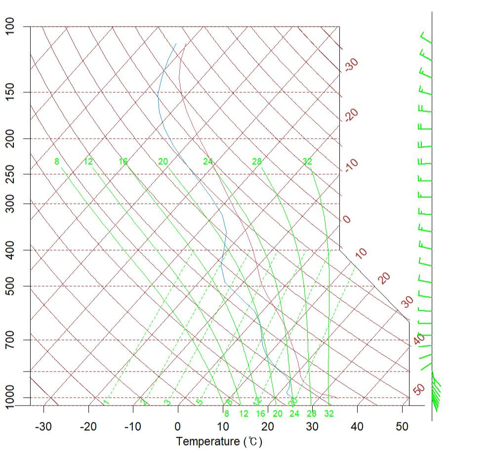
참고 문헌
[논문]
- 없음
[보고서]
- 없음
[URL]
- 없음
문의사항
[기상학/프로그래밍 언어]
- sangho.lee.1990@gmail.com
[해양학/천문학/빅데이터]
- saimang0804@gmail.com
'프로그래밍 언어 > R' 카테고리의 다른 글
| [R] 온라인 리눅스 (Linux) 환경에서 R 및 R Studio 설치/업데이트 (0) | 2021.01.27 |
|---|---|
| [R] 끄투 자동 게임 수행 프로그램 (test) (11) | 2021.01.22 |
| [R] 시정거리 자료를 이용한 한반도 지역 등고선 (Contour) 시각화 및 해양 마스킹 (2) | 2021.01.17 |
| [R] 베이지안 선형회귀 모델을 통한 ASOS 종관 기상 관측지점 자료를 이용하여 AWS 관측 지점의 기온 추정 (0) | 2021.01.17 |
| [R] 구글 번역 API 및 R 프로그램을 이용하여 마인크래프트 1.12.1 모드 파일 자동으로 번역 후 적용하기 (구글 API 신청 방법 포함) (0) | 2020.12.28 |