[R] sf 패키지를 이용한 지도 투영법 소개 및 가시화

정보

업무명 : sf 패키지를 이용한 지도 투영법 소개 및 가시화
작성자 : 이상호
작성일 : 2020-03-05
설 명 :
수정이력 :

내용

[개요]

안녕하세요? 기상 연구 및 웹 개발을 담당하고 있는 해솔입니다.
지도 투영은 지구 표면을 평면으로 평면화하여 지도를 만드는 방법입니다. 이를 위해서는 지구 표면에서 평면 위의 위치로 위도 및 경도의 위치를 체계적으로 변환해야합니다.
일반적으로 평면에서 구의 모든 돌출은 표면을 어느 정도 왜곡시킵니다. 지도의 목적에 따라 일부 왜곡이 허용되거나 다른 왜곡이 허용되지 않습니다.
따라서 일부 왜곡됨에도 불구하고 구형 본체의 일부 특성을 보존하기 위해 맵 투영이 존재한다. 투영은 보존하는 모델의 속성에 따라 그룹화됩니다. 보다 일반적인 범주 중 일부는 다음과 같습니다.
- 원통형 (예 : Mercator)
- 원추형 (예 : Albers)
- 평면형 (예 : Stereographic)
3개의 개발 가능한 표면 (평면, 원통, 원뿔)은 지도 투영을 이해하고 설명하고 개발하는 데 유용한 모델을 제공합니다. 그러나 이러한 모델은 2가지 기본 방식으로 제한됩니다.
우선 사용중인 대부분의 세계 예측은 이러한 범주에 속하지 않습니다. 즉 이러한 범주에 속하는 대부분의 예측조차도 물리적 투영을 통해 자연스럽게 달성할 수 없습니다.
따라서 sf 패키지를 통해 널리 사용되는 투영법을 소개해드리고자 합니다.

[특징]

지도 투영법을 이해하기 위해서 sf 패키지가 요구되며 이 프로그램은 이러한 목적을 달성하기 위한 소프트웨어

[기능]

sf 패키지 소개

[활용 자료]

자료 설명 : 세계 지도 자료
세부 정보 : 11개 변수에서 177개 국가 레코드 포함
제공처 : spData 패키지
자세한 내용은 소스 코드 참조

[자료 처리 방안 및 활용 분석 기법]

없음

[사용법]

소스 코드 참조

[사용 OS]

Windows 10

[사용 언어]

R v3.6.2
R Studio v1.2.5033

소스 코드

[명세]

전역 설정
- 최대 10 자리 설정
- 메모리 해제
- 영어 인코딩 설정
- 가시화에 필요한 폰트 설정 (다운로드 링크 참조)

[블로그 관리] 코딩/발표자료를 위한 폰트 : Apple 산돌고딕, Monaco 맑은고딕, Palatino Linotype, New Century Schoolbook, Playfair Display Regular, KoPubWor

정보 업무명 : 코딩/발표 자료를 위한 폰트 제공 작성자 : 이상호 작성일 : 2019-12-28 설 명 : 수정이력 : 폰트 설명 [Apple 산돌고딕 Neo] [Monaco 맑은고딕] [Palatino Linotype] [New Century Schoolbook]..

shlee1990.tistory.com

# Set Option
options(digits = 10)
memory.limit(size = 9999999999999)
Sys.setlocale("LC_TIME", "english")
font = "Palatino Linotype"

라이브러리 읽기
- sf : 간단한 기능, 점, 선 및 다각형을 지원
- tidyverse : 데이터 조작 기능 제공
- ggplot2 : 가시화 제공

# Library Load
library(sf)
library(tidyverse)
library(spData)
library(extrafont)
library(metR)
library(ggplot2)

세계 지도 읽기
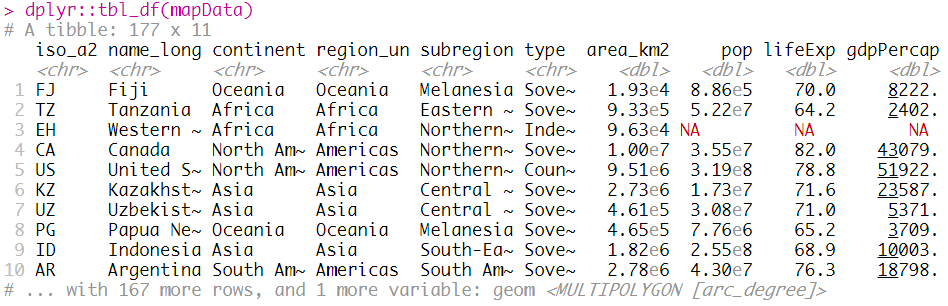
- spData 패키지에서 제공되는 세계 지도 데이터를 사용
- 이러한 데이터 세트는 11개의 변수에서 177 개 국가의 레코드를 포함

# set Map Data
mapData = sf::st_as_sf(spData::world)

dplyr::tbl_df(mapData)

EPSG 코드
- EPSG 코드는 GCS (Geographical Coordinate System) 좌표 변환 및 해당 구성 요소에 지정
- 특정 좌표계에 대한 모든 세부 사항을 기억하는 대신 간단히 epsg 코드를 통해 투영 및 변환 가능
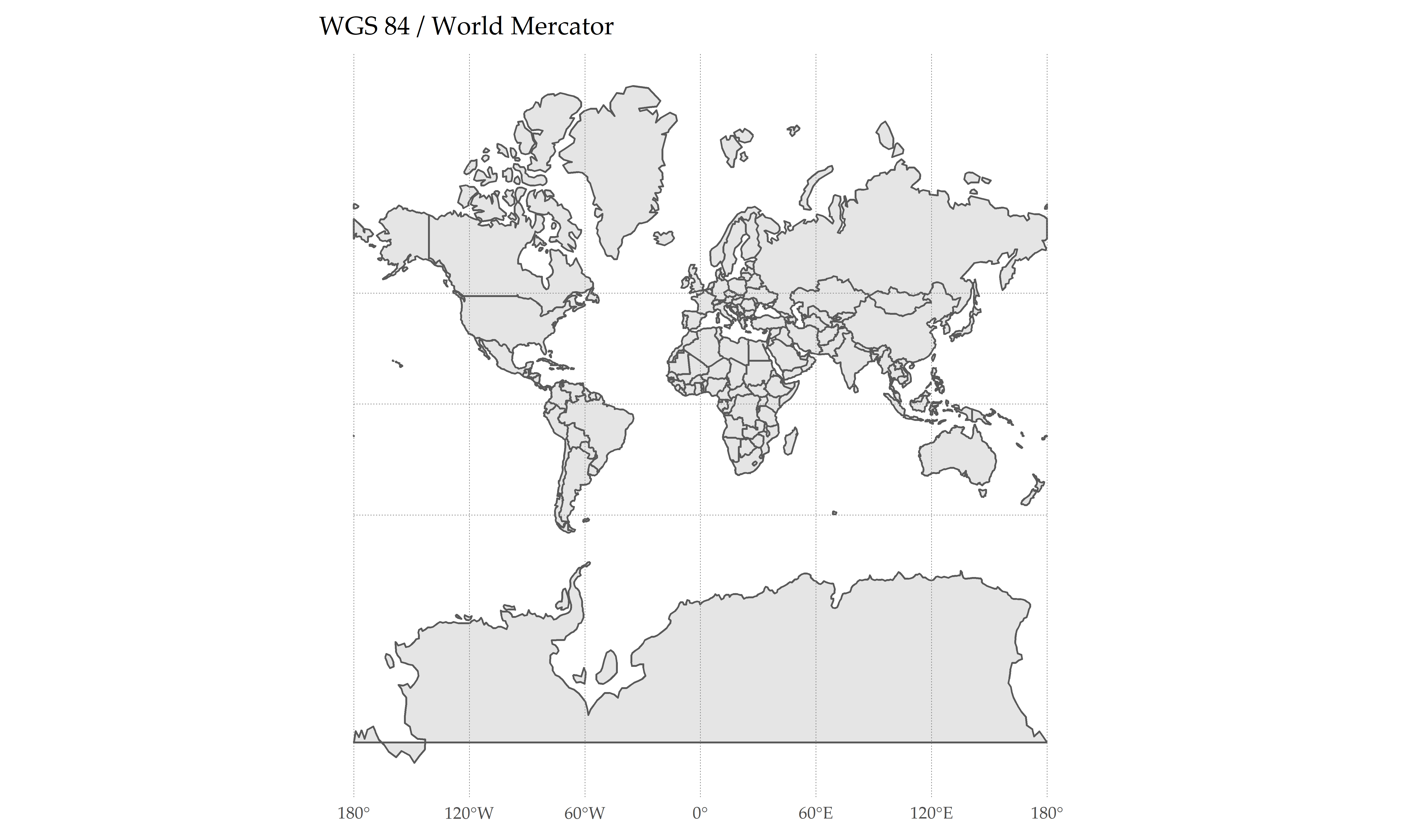
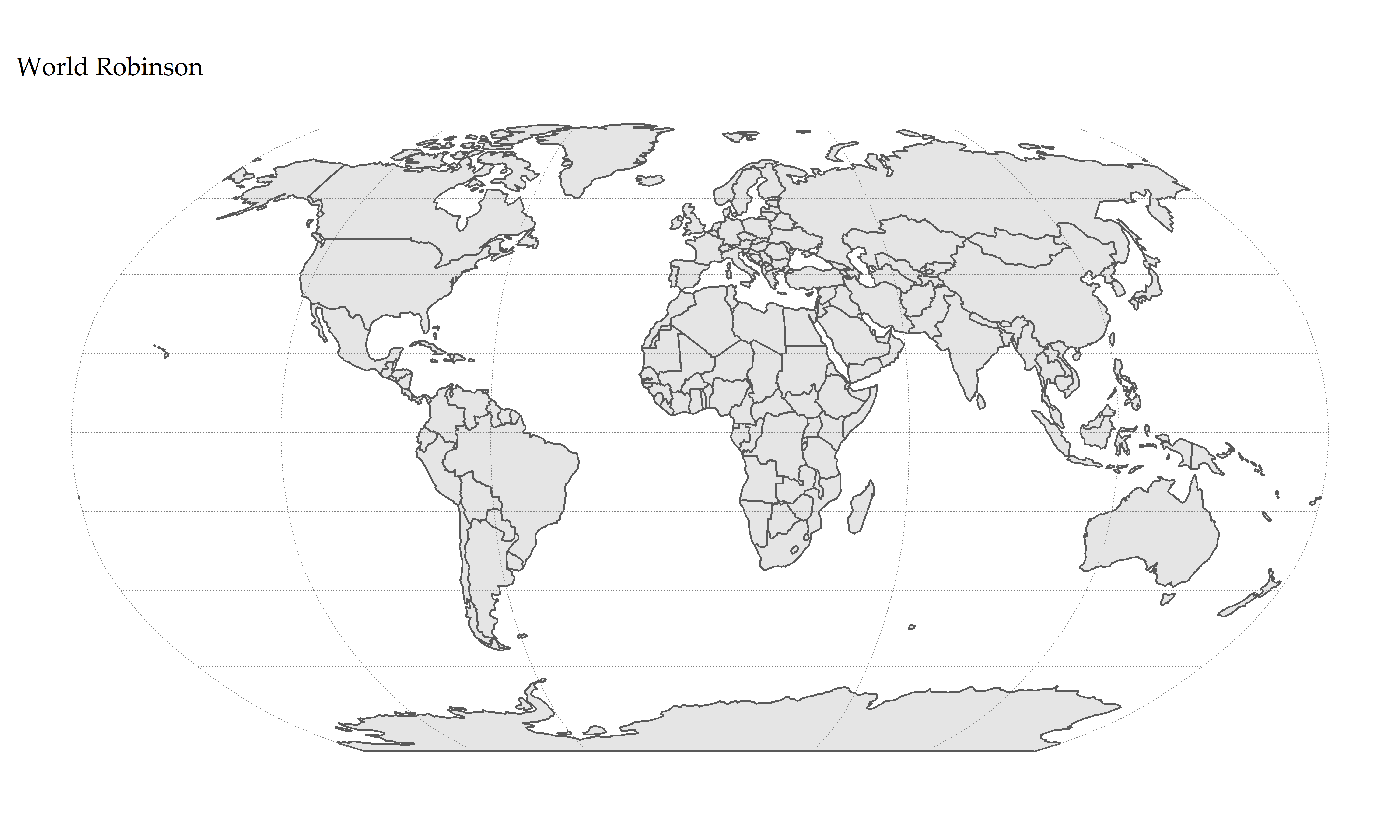
- 아래는 다양한 투영법에 따라 가시화 결과

# WGS 84 - WGS84 - World Geodetic System 1984, used in GPS
ggplot() +
    ggspatial::layer_spatial(data = mapData) +
    coord_sf(crs = 4326) +
    ggtitle("WGS 84 - WGS84 - World Geodetic System 1984, used in GPS") +
    metR:::theme_field() +
    theme(text = element_text(family = font)) +
    ggsave(filename = paste0("FIG/MAP/WGS 84 - WGS84 - World Geodetic System 1984, used in GPS.png"), width = 10, height = 6, dpi = 600)

# WGS 84 / World Mercator
ggplot() +
    ggspatial::layer_spatial(data = mapData) +
    coord_sf(crs = 3395) +
    ggtitle("WGS 84 / World Mercator") +
    metR:::theme_field() +
    theme(text = element_text(family = font)) +
    ggsave(filename = paste0("FIG/MAP/WGS 84 World Mercator.png"), width = 10, height = 6, dpi = 600)

# WGS 84 / World Equidistant Cylindrical
ggplot() +
    ggspatial::layer_spatial(data = mapData)+
    coord_sf(crs = 4087) +
    ggtitle("WGS 84 / World Equidistant Cylindrical")+
    metR:::theme_field() +
    theme(text = element_text(family = font)) +
    ggsave(filename = paste0("FIG/MAP/World Equidistant Cylindrical.png"), width = 10, height = 6, dpi = 600)

# World Equidistant Cylindrical (Sphere)
ggplot() +
    ggspatial::layer_spatial(data = mapData)+
    coord_sf(crs = 4088) +
    ggtitle("World Equidistant Cylindrical (Sphere)")+
    metR:::theme_field() +
    theme(text = element_text(family = font)) +
    ggsave(filename = paste0("FIG/MAP/World Equidistant Cylindrical (Sphere).png"), width = 10, height = 6, dpi = 600)

# World Robinson
ggplot() +
    ggspatial::layer_spatial(data = mapData)+
    coord_sf(crs = 54030) +
    ggtitle("World Robinson") +
    metR:::theme_field() +
    theme(text = element_text(family = font)) +
    ggsave(filename = paste0("FIG/MAP/World Robinson.png"), width = 10, height = 6, dpi = 600)

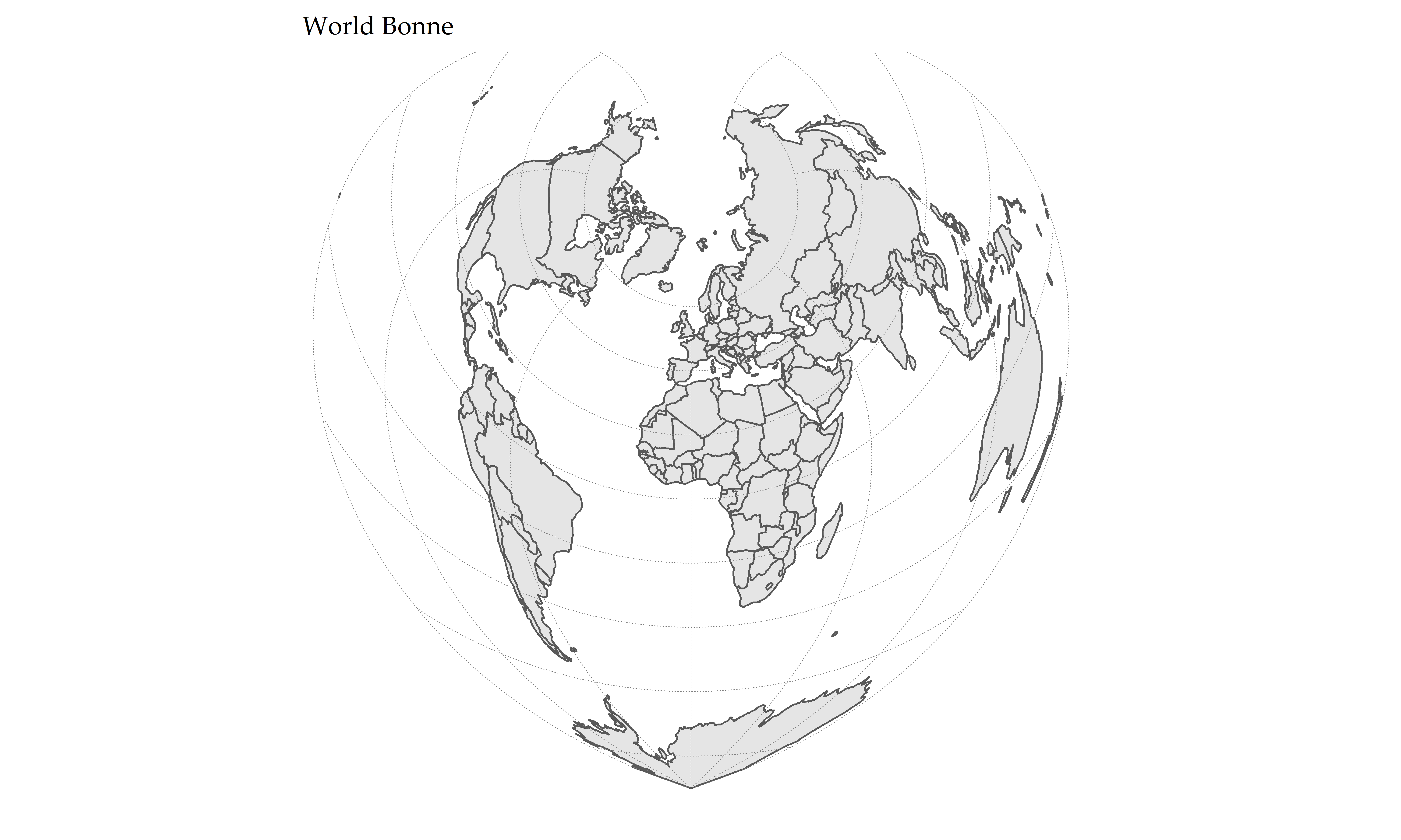
# World Bonne
ggplot() +
    ggspatial::layer_spatial(data = mapData)+
    coord_sf(crs = 54024) +
    ggtitle("World Bonne")+
    metR:::theme_field() +
    theme(text = element_text(family = font)) +
    ggsave(filename = paste0("FIG/MAP/World Bonne.png"), width = 10, height = 6, dpi = 600)

# World Polyconic
ggplot() +
    ggspatial::layer_spatial(data = mapData)+
    coord_sf(crs = 54021) +
    ggtitle("World Polyconic") +
    cowplot::theme_minimal_grid() +
    metR:::theme_field() +
    theme(text = element_text(family = font)) +
    ggsave(filename = paste0("FIG/MAP/Polyconic.png"), width = 10, height = 6, dpi = 600)

# World Mollweide
ggplot() +
    geom_sf(data = mapData) +
    coord_sf(crs = 54009) +
    ggtitle("World Mollweide") +
    metR:::theme_field() +
    theme(text = element_text(family = font)) +
    ggsave(filename = paste0("FIG/MAP/Mollweide.png"), width = 10, height = 6, dpi = 600)

# World Azimuthal Equidistant
ggplot() +
    ggspatial::layer_spatial(data = mapData) +
    coord_sf(crs = 54032) +
    ggtitle("World Azimuthal Equidistant") 
    metR:::theme_field() +
    theme(text = element_text(family = font)) +
        ggsave(filename = paste0("FIG/MAP/World Azimuthal Equidistant.png"), width = 10, height = 6, dpi = 600)

# World Azimuthal Equidistant
ggplot() +
    ggspatial::layer_spatial(data = mapData) +
    coord_sf(crs = 54032) +
    ggtitle("World Azimuthal Equidistant") 
    metR:::theme_field() +
    theme(text = element_text(family = font)) +
        ggsave(filename = paste0("FIG/MAP/World Azimuthal Equidistant.png"), width = 10, height = 6, dpi = 600)

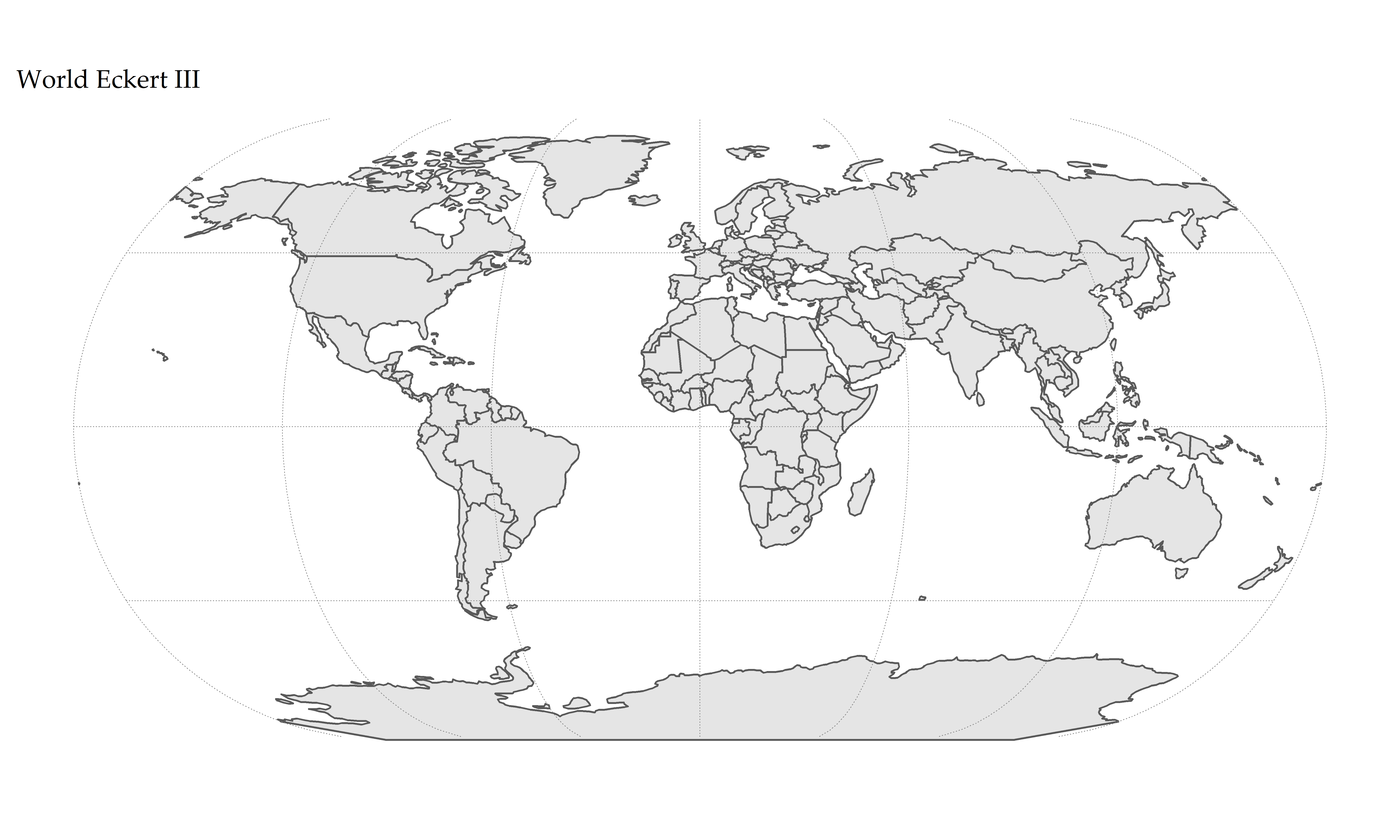
# World Eckert III
ggplot() +
    ggspatial::layer_spatial(data = mapData) +
    coord_sf(crs = 54013) +
    ggtitle("World Eckert III") +
    metR:::theme_field() +
    theme(text = element_text(family = font))  +
    ggsave(filename = paste0("FIG/MAP/World Eckert III.png"), width = 10, height = 6, dpi = 600)

# World Eckert IV
ggplot() +
    ggspatial::layer_spatial(data = dunia) +
    coord_sf(crs = 54012) +
    ggtitle("World Eckert IV") +
    metR:::theme_field() +
    theme(text = element_text(family = font)) +
    ggsave(filename = paste0("FIG/MAP/World Eckert IV.png"), width = 10, height = 6, dpi = 600)

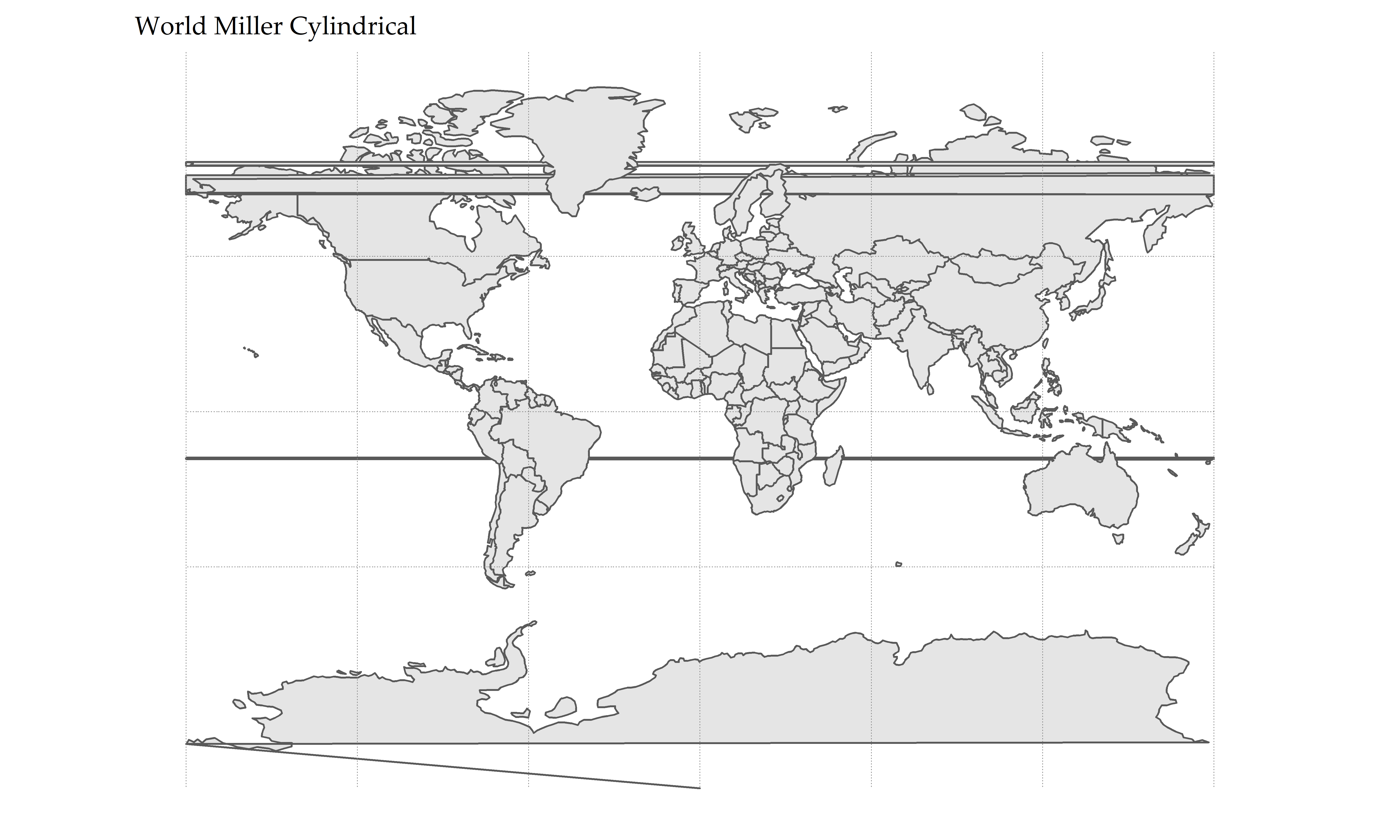
# World Miller Cylindrical
ggplot() +
    ggspatial::layer_spatial(data = dunia) +
    coord_sf(crs = 54003) +
    ggtitle("World Miller Cylindrical") +
    metR:::theme_field() +
    theme(text = element_text(family = font)) +
    ggsave(filename = paste0("FIG/MAP/World Miller Cylindrical.png"), width = 10, height = 6, dpi = 600)

# World Equidistant Cylindrical
ggplot() +
    ggspatial::layer_spatial(data = dunia) +
    coord_sf(crs = 54002) +
    ggtitle("World Equidistant Cylindrical") +
    metR:::theme_field() +
    theme(text = element_text(family = font)) +
    ggsave(filename = paste0("FIG/MAP/World Equidistant Cylindrical.png"), width = 10, height = 6, dpi = 600)

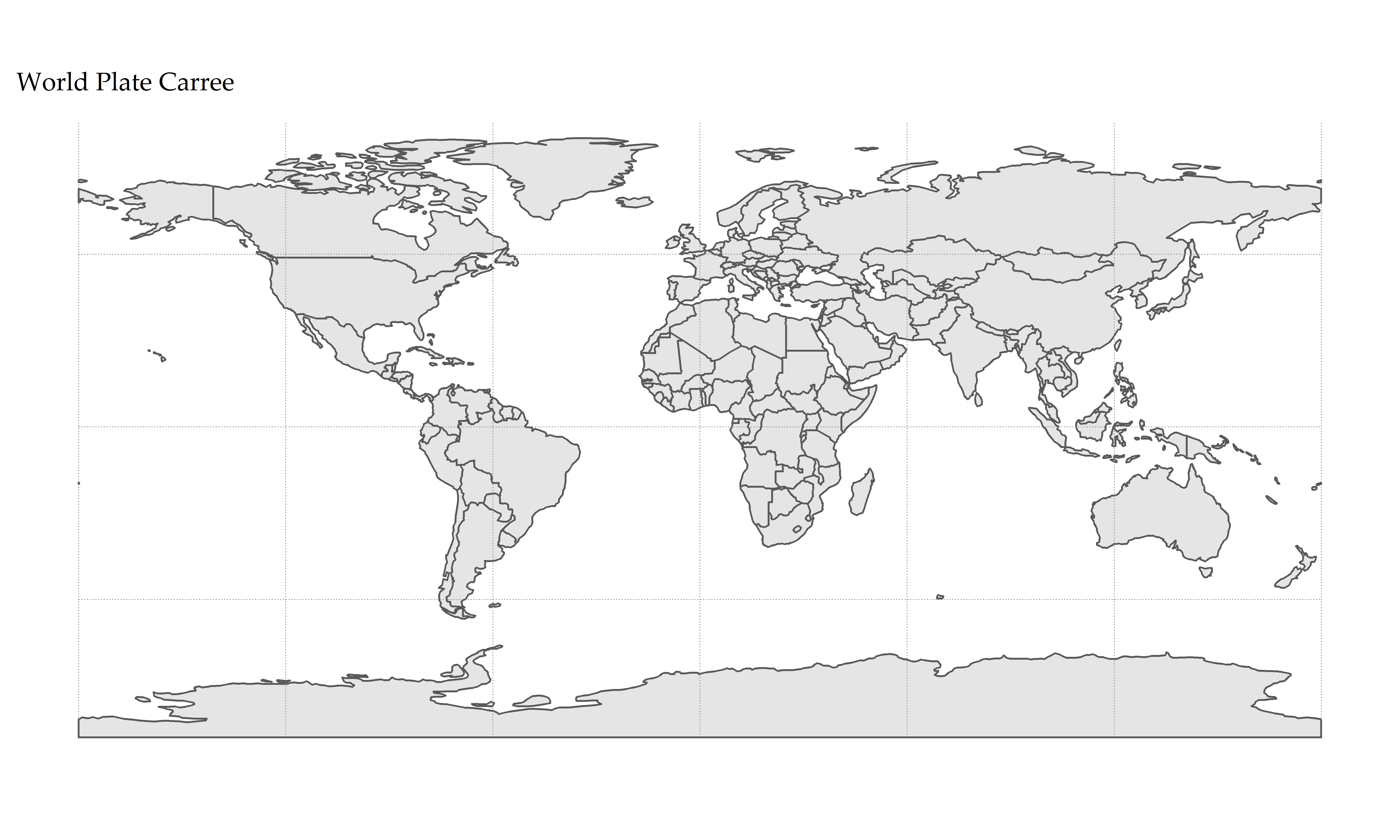
# World Plate Carree
ggplot() +
    ggspatial::layer_spatial(data = dunia) +
    coord_sf(crs = 54001) +
    ggtitle("World Plate Carree")+
    metR:::theme_field() +
    theme(text = element_text(family = font))  +
    ggsave(filename = paste0("FIG/MAP/World Plate Carree.png"), width = 10, height = 6, dpi = 600)

# World Two Point Equidistant
ggplot() +
    ggspatial::layer_spatial(data = dunia)+
    coord_sf(crs = 54031) +
    ggtitle("World Two Point Equidistant")+
    metR:::theme_field() +
    theme(text = element_text(family = font))  +
    ggsave(filename = paste0("FIG/MAP/World Two Point Equidistant.png"), width = 10, height = 6, dpi = 600)

[전체]

참고 문헌

[논문]

없음

[보고서]

없음

[URL]

없음

문의사항

[기상학/프로그래밍 언어]

sangho.lee.1990@gmail.com

[해양학/천문학/빅데이터]

saimang0804@gmail.com

저작자표시 비영리 변경금지

'프로그래밍 언어 > R' 카테고리의 다른 글

[R] "ncdf4" 패키지 및 NetCDF 형식인 NOAA 최적 내삽 자료를 이용하여 데이터 프레임 (Data Frame)으로 변환 처리 및 가시화 (2) (0)	2020.03.08
[R] "raster" 패키지 및 NetCDF 형식인 NOAA 최적 내삽 자료를 이용하여 데이터 프레임 (Data Frame)으로 변환 처리 및 가시화 (1) (0)	2020.03.07
[R] 시/공간 자료 처리 및 분석 (Handling and Analyzing Spatio-Temporal Data) 패키지 소개 (0)	2020.03.05
[R] 상자그림을 다채롭게 보여주는 "lvplot" 패키지 (0)	2020.03.03
[R] 덴드로그램 플롯의 레이블에 색을 입혀주는 "colorhcplot" 패키지 (0)	2020.03.03

정보

내용