[Python] 파이썬 NetCDF 형식인 Aqua/CERES 기상위성 자료를 이용한 가시화

정보
내용
소스 코드
참고 문헌
문의사항

정보

업무명 : NetCDF 형식인 Aqua/CERES 기상위성 자료를 이용한 가시화
작성자 : 이상호
작성일 : 2019-10-22
설 명 :
수정이력 :
- 2020-02-05 : 소스 코드 명세 추가

내용

[개요]

안녕하세요? 웹 개발 및 연구 개발을 담당하고 있는 해솔입니다.
최근 국외 기상학회에서는 R 또는 Python을 통해 가시화 결과를 종종 볼 수 있습니다.
따라서 Python을 이용하여 NetCDF 자료 전처리 및 가시화를 소개해 드리고자 합니다.

[특징]

NetCDF 형태인 기상위성 자료를 이해하기 위해 가시화 도구가 필요하며 이 프로그램은 이러한 목적을 달성하기 위해 고안된 소프트웨어

[기능]

Aqua/CERES 기상위성 자료를 이용한 가시화

[활용 자료]

위성명 : Aqua 기상위성
센서명 : CERES
자료종류 : 대기상단에서의 상향단파복사
영역 : 전지구 및 전구
해상도 : 20 km
확장자 : .nc
기간 : 2015년 07월 15일 0000-2300 UTC

[자료 처리 방안 및 활용 분석 기법]

없음

[사용법]

입력 자료를 동일 디렉터리 위치
소스 코드를 실행 (Jupyter notebook 실행)
가시화 결과를 확인

[사용 OS]

Window 10

[사용 언어]

Python v2.7

소스 코드

[명세]

라이브러리 읽기
- NetCDF 읽기 : netCDF4
- 데이터 전처리 : dplython
- 가시화 : matplot

# Library
import pandas as pd
import numpy as np
import sys 
# import iris
import os
import matplotlib.pyplot as plt
from dplython import *
    # (DplyFrame, X, diamonds, select, sift, sample_n,
    #     sample_frac, head, arrange, mutate, group_by, summarize, DelayFunction) 
from scipy.stats import linregress
from matplotlib import pyplot as plt
from IPython.display import Image
from mpl_toolkits.basemap import Basemap
from matplotlib.colors import Normalize
import matplotlib
import matplotlib.cm as cm
import seaborn as sns
from scipy.stats import linregress
from matplotlib import rcParams
from netCDF4 import Dataset
import struct
import binascii
from mpl_toolkits.basemap import addcyclic
from netCDF4 import num2date, date2num, date2index
import datetime
from pyhdf.SD import SD, SDC
import h5py

NetCDF 파일 읽기

ncfile_path  = 'CERES/CERES_SSF_Aqua-XTRK_Edition4A_Subset_2015071500-2015071523.nc'
ncfile = Dataset(ncfile_path)

# print(ncfile)

NetCDF 헤더 보기
- 원도우 (Window)에서 ncdump를 사용할 경우 Anaconda Cloud에서 "conda install -c anaconda netcdf4" 설치 필요
- ncdump 외에 "ncBrowse", "Panoply" 등 다양한 도구가 있으니 참고 바램

[연구개발] NetCDF 파일을 이용한 시각화 도구 소개

정보 업무명 : NetCDF 파일을 이용한 시각화 도구 소개 작성자 : 이상호 작성일 : 2020-02-03 설 명 : 수정이력 : 내용 [개요] 안녕하세요? 기상 연구 및 웹 개발을 담당하고 있는 해솔입니다. NetCDF 파일 (*.nc)..

shlee1990.tistory.com

!ncdump -h CERES/CERES_SSF_Aqua-XTRK_Edition4A_Subset_2015071500-2015071523.nc

netcdf CERES/CERES_SSF_Aqua-XTRK_Edition4A_Subset_2015071500-2015071523 {
dimensions:
	time = UNLIMITED ; // (2370473 currently)
	The_8_most_prevalent_surface_types = 8 ;
	Conditions_clear__lower__upper__upper_over_lower = 4 ;
variables:
	double time(time) ;
		time:long_name = "time" ;
		time:units = "days since 1970-01-01 00:00:00" ;
		time:_FillValue = 1.79769313486232e+308 ;
		time:valid_range = 0., 39412.5 ;
	float lon(time) ;
		lon:long_name = "longitude" ;
		lon:units = "degrees_east" ;
		lon:_FillValue = 3.402823e+038f ;
		lon:valid_range = -180.f, 180.f ;
	float lat(time) ;
		lat:long_name = "latitude" ;
		lat:units = "degrees_north" ;
		lat:_FillValue = 3.402823e+038f ;
		lat:valid_range = -90.f, 90.f ;
	double Time_of_observation(time) ;
		Time_of_observation:orig_name = "Time of observation" ;
		Time_of_observation:units = "day" ;
		Time_of_observation:format = "F18.9" ;
		Time_of_observation:_FillValue = 1.79769313486232e+308 ;
		Time_of_observation:valid_range = 2440000., 2480000. ;
	float Longitude_of_CERES_FOV_at_surface(time) ;
		Longitude_of_CERES_FOV_at_surface:orig_name = "Longitude of CERES FOV at surface" ;
		Longitude_of_CERES_FOV_at_surface:units = "degrees" ;
		Longitude_of_CERES_FOV_at_surface:format = "F18.9" ;
		Longitude_of_CERES_FOV_at_surface:_FillValue = 3.402823e+038f ;
		Longitude_of_CERES_FOV_at_surface:valid_range = 0.f, 360.f ;
	float Colatitude_of_CERES_FOV_at_surface(time) ;
		Colatitude_of_CERES_FOV_at_surface:orig_name = "Colatitude of CERES FOV at surface" ;
		Colatitude_of_CERES_FOV_at_surface:units = "degrees" ;
		Colatitude_of_CERES_FOV_at_surface:format = "F18.9" ;
		Colatitude_of_CERES_FOV_at_surface:_FillValue = 3.402823e+038f ;
		Colatitude_of_CERES_FOV_at_surface:valid_range = 0.f, 180.f ;
	float CERES_solar_zenith_at_surface(time) ;
		CERES_solar_zenith_at_surface:orig_name = "CERES solar zenith at surface" ;
		CERES_solar_zenith_at_surface:units = "degrees" ;
		CERES_solar_zenith_at_surface:format = "F18.9" ;
		CERES_solar_zenith_at_surface:_FillValue = 3.402823e+038f ;
		CERES_solar_zenith_at_surface:valid_range = 0.f, 180.f ;
	float CERES_SW_TOA_flux___upwards(time) ;
		CERES_SW_TOA_flux___upwards:orig_name = "CERES SW TOA flux - upwards" ;
		CERES_SW_TOA_flux___upwards:units = "Watts per square meter" ;
		CERES_SW_TOA_flux___upwards:format = "F18.9" ;
		CERES_SW_TOA_flux___upwards:_FillValue = 3.402823e+038f ;
		CERES_SW_TOA_flux___upwards:valid_range = 0.f, 1400.f ;
	float TOA_Incoming_Solar_Radiation(time) ;
		TOA_Incoming_Solar_Radiation:orig_name = "TOA Incoming Solar Radiation" ;
		TOA_Incoming_Solar_Radiation:units = "Watts per square meter" ;
		TOA_Incoming_Solar_Radiation:format = "F18.9" ;
		TOA_Incoming_Solar_Radiation:_FillValue = 3.402823e+038f ;
		TOA_Incoming_Solar_Radiation:valid_range = 0.f, 1400.f ;
	float CERES_downward_SW_surface_flux___Model_B(time) ;
		CERES_downward_SW_surface_flux___Model_B:orig_name = "CERES downward SW surface flux - Model B" ;
		CERES_downward_SW_surface_flux___Model_B:units = "Watts per square meter" ;
		CERES_downward_SW_surface_flux___Model_B:format = "F18.9" ;
		CERES_downward_SW_surface_flux___Model_B:_FillValue = 3.402823e+038f ;
		CERES_downward_SW_surface_flux___Model_B:valid_range = 0.f, 1400.f ;
	short Surface_type_index(time, The_8_most_prevalent_surface_types) ;
		Surface_type_index:orig_name = "Surface type index" ;
		Surface_type_index:units = "N/A" ;
		Surface_type_index:format = "I10" ;
		Surface_type_index:_FillValue = 32767s ;
		Surface_type_index:valid_range = 1s, 20s ;
	float Clear_layer_overlap_percent_coverages(time, Conditions_clear__lower__upper__upper_over_lower) ;
		Clear_layer_overlap_percent_coverages:orig_name = "Clear/layer/overlap percent coverages" ;
		Clear_layer_overlap_percent_coverages:units = "N/A" ;
		Clear_layer_overlap_percent_coverages:format = "F18.9" ;
		Clear_layer_overlap_percent_coverages:_FillValue = 3.402823e+038f ;
		Clear_layer_overlap_percent_coverages:valid_range = 0.f, 100.f ;

// global attributes:
		:Conventions = "CF-1.0" ;
		:Subsetter_title = "ASDC CERES Subset" ;
		:Subsetter_version = "2.9.b1" ;
		:Subsetter_institution = "Atmospheric Science Data Center (ASDC) http://eosweb.larc.nasa.gov" ;
		:Subsetter_history = "2017-08-03T10:35:23 -0400 SubsetCeresSsf" ;
		:Subsetter_temporalFilter = "2015-07-15T00:00:00.000000Z to 2015-07-15T23:59:59.000000Z" ;
		:Subsetter_spatialFilter = "POLYGON ((-180 -90, -180 90, 180 90, 180 -90, -180 -90))" ;
		:Subsetter_parameterFilter = "none" ;
		:platform = "Aqua" ;
		:history = "Thu Aug  3 11:30:59 2017: ncrcat -o CERES_SSF_Aqua-XTRK_Edition4A_Subset_2015071500-2015071523.nc" ;
		:nco_input_file_number = 24 ;
		:nco_input_file_list = "CER_SSF_Aqua-FM3-MODIS_Edition4A_401404.2015071500_Subset.nc CER_SSF_Aqua-FM3-MODIS_Edition4A_401404.2015071501_Subset.nc CER_SSF_Aqua-FM3-MODIS_Edition4A_401404.2015071502_Subset.nc CER_SSF_Aqua-FM3-MODIS_Edition4A_401404.2015071503_Subset.nc CER_SSF_Aqua-FM3-MODIS_Edition4A_401404.2015071504_Subset.nc CER_SSF_Aqua-FM3-MODIS_Edition4A_401404.2015071505_Subset.nc CER_SSF_Aqua-FM3-MODIS_Edition4A_401404.2015071506_Subset.nc CER_SSF_Aqua-FM3-MODIS_Edition4A_401404.2015071507_Subset.nc CER_SSF_Aqua-FM3-MODIS_Edition4A_401404.2015071508_Subset.nc CER_SSF_Aqua-FM3-MODIS_Edition4A_401404.2015071509_Subset.nc CER_SSF_Aqua-FM3-MODIS_Edition4A_401404.2015071510_Subset.nc CER_SSF_Aqua-FM3-MODIS_Edition4A_401404.2015071511_Subset.nc CER_SSF_Aqua-FM3-MODIS_Edition4A_401404.2015071512_Subset.nc CER_SSF_Aqua-FM3-MODIS_Edition4A_401404.2015071513_Subset.nc CER_SSF_Aqua-FM3-MODIS_Edition4A_401404.2015071514_Subset.nc CER_SSF_Aqua-FM3-MODIS_Edition4A_401404.2015071515_Subset.nc CER_SSF_Aqua-FM3-MODIS_Edition4A_401404.2015071516_Subset.nc CER_SSF_Aqua-FM3-MODIS_Edition4A_401404.2015071517_Subset.nc CER_SSF_Aqua-FM3-MODIS_Edition4A_401404.2015071518_Subset.nc CER_SSF_Aqua-FM3-MODIS_Edition4A_401404.2015071519_Subset.nc CER_SSF_Aqua-FM3-MODIS_Edition4A_401404.2015071520_Subset.nc CER_SSF_Aqua-FM3-MODIS_Edition4A_401404.2015071521_Subset.nc CER_SSF_Aqua-FM3-MODIS_Edition4A_401404.2015071522_Subset.nc CER_SSF_Aqua-FM3-MODIS_Edition4A_401404.2015071523_Subset.nc" ;
		:nco_openmp_thread_number = 1 ;
}

변수 설정
- NetCDF에서 필요한 변수 저장
  - 시간 : 시간 변수 (times), 단위 (dtime), Data Frame 형태로 변환 (time)
  - 변수 : 위도 (lon), 경도 (lat), 태양 천정각 (sza), 대기 상단에서의 하향 단파복사 (insw), 대기 상단에서의 상향단파복사 (rsr), 지표면에서의 하향 단파복사 (dsr), 지표면 특성 (surface_type), 청천 비율 (clear_fraction)

# Time
times = ncfile.variables[u'time']
dtime = num2date(times[:], times.units)
time = pd.to_datetime(dtime)

# Variable
lon  = ncfile.variables[u'lon'][:] 
lat  = ncfile.variables[u'lat'][:] 
sza  = ncfile.variables[u'CERES_solar_zenith_at_surface'][:]
insw = ncfile.variables[u'TOA_Incoming_Solar_Radiation'][:]
rsr  = ncfile.variables[u'CERES_SW_TOA_flux___upwards'][:]
dsr  = ncfile.variables[u'CERES_downward_SW_surface_flux___Model_B'][:]
surface_type   = ncfile.variables[u'Surface_type_index'][:,1]
clear_fraction = ncfile.variables[u'Clear_layer_overlap_percent_coverages'][:,1]

Data Frame 설정
- 시간의 경우 년, 월, 일, 시, 분, 초, 마이크로초로 변환
- 앞서 설명한 변수에 대한 컬럼명 지정

data =  pd.DataFrame( np.column_stack([time.year, time.month, time.day, 
                                       time.hour, time.minute, time.second, time.microsecond, 
                                       lon, lat, sza, insw, rsr, dsr, surface_type, clear_fraction]),
                     columns=['year', 'month', 'day', 'hour', 'minute', 'second', 'microsecond', 
                              'lon', 'lat', 'sza', 'insw', 'rsr', 'dsr', 'surface_type', 'clear_fraction'])

data.head()

Data Frame를 통해 L1 전처리
- 최근 데이터 분석에서 사용되는 R의 "dplyr" 라이브러리와 유사한 "dplython"를 사용
- 각 변수에 대해 최대값 및 최소값 설정

data_L1 = ( DplyFrame(data) >>
           sift( (-90 <= X.lat)   &  (X.lat <= 90) ) >>
           sift( (-180 <= X.lon)  &  (X.lon <= 180) ) >>
           sift( (0 <= X.rsr)  &  (X.rsr <= 1400) ) >>
           sift( (0 <= X.dsr)  &  (X.dsr <= 1400) ) >>
           sift( (0 <= X.insw) &  (X.insw <= 1400) ) >>
           sift( (0 <= X.sza)  &  (X.sza <= 90) ) >>
           sift( (0 <= X.hour)  &  (X.hour <= 23) )
        )

data_L1.head()

	year	month	day	hour	minute	second	microsecond	lon	lat	sza	insw	rsr	dsr	surface_type	clear_fraction
1	2015.0	7.0	15.0	0.0	0.0	0.0	63770.0		74.017220	66.208206	77.034363	295.658325	116.962135	98.196671	10.0	73.008736
2	2015.0	7.0	15.0	0.0	0.0	0.0	73788.0		73.517990	66.443062	77.118500	293.772278	117.117500	93.707993	17.0	72.541275
3	2015.0	7.0	15.0	0.0	0.0	0.0	93784.0		72.567398	66.873962	77.275452	290.252289	94.097664	104.814674	7.0	39.283241
4	2015.0	7.0	15.0	0.0	0.0	0.0	113779.0	71.685020	67.255684	77.417488	287.064911	76.625443	125.678894	17.0	41.375149
5	2015.0	7.0	15.0	0.0	0.0	0.0	133775.0	70.850426	67.601425	77.548729	284.118256	121.472298	86.047745	17.0	81.676659

가시화를 위한 설정

- 초기 설정
  - 크기 : figure
  - 스타일 : style
  - 폰트 : rc, rcParams
  - 지도 해상도 : Basemap

- 변수 설정
  - 위도 (lon), 경도 (lat), 상향단파복사 (rsr)
- 그림 설정
  - 산점도 : scatter
  - 컬러바 : colorbar
  - 해안선 : drawcostlines, drawcountries, drawmapboundary
  - 수평/수직 그리드 : drawparallels, drawmeridians
  - 그림 제목 : title
  - 그림 저장 : savefig

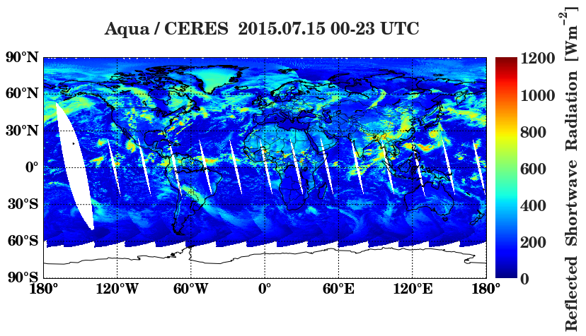
%matplotlib inline
# define plot size in inches (width, height) & resolution(DPI)
plt.figure(figsize=(12, 10))

# style
plt.style.use('seaborn-darkgrid')

# define font size
plt.rc("font", size=20)
plt.rcParams['font.family'] = 'New Century Schoolbook'
# rcParams['font.family'] = 'sans-serif'
# plt.rcParams["font.weight"] = "bold"
# plt.rcParams['axes.labelsize'] = 22
# plt.rcParams['xtick.labelsize'] = 22
# plt.rcParams['ytick.labelsize'] = 22
# plt.rcParams["axes.labelweight"] = "bold"
# plt.rcParams["axes.titleweight"] = "bold"

m = Basemap(projection='cyl', lon_0 = 0, lat_0 = 0)
# c (crude) < l (low) < i (intermediate) < h (high) < f (full)
# Source: http://seesaawiki.jp/met-python/d/Basemap

X, Y = m(data_L1.lon.values, data_L1.lat.values)
VAL  = data_L1.rsr.values
# print(VAL)

m.scatter(X, Y, c=VAL, s=1.0, marker="s", zorder=1, vmin=0, vmax=1200, cmap=plt.cm.get_cmap('jet'), alpha=1.0) 
m.colorbar(location='right', label='Reflected  Shortwave  Radiation  $\mathregular{[Wm^{-2}]}$')

m.drawcoastlines()
m.drawcountries()
m.drawmapboundary(fill_color='white')
m.drawparallels(np.arange(-90,91,30),labels=[1,0,0,0],dashes=[2,2])
m.drawmeridians(np.arange(0,361,60),labels=[0,0,0,1],dashes=[2,2]) 

plt.title('Aqua / CERES  2015.07.15 00-23 UTC \n')
# plt.savefig("FIG/Scane_analysis_Himawari-8_AHI_RSR.png")
plt.show()

etc-image-2 — 그림. Aqua/CERES 기상위성 자료를 이용한 대기상단에서의 상향단파복사 가시화 (전지구).

matplotlib를 이용한 가시화
- 초기 설정
- 변수 설정
- 그림 설정
  - 그림 좌표에서 원하는 글자 넣기 : annotate

%matplotlib inline
# define plot size in inches (width, height) & resolution(DPI)
plt.figure(figsize=(12, 10))

# style
plt.style.use('seaborn-darkgrid')

# define font size
plt.rc("font", size=22)
plt.rcParams['font.family'] = 'New Century Schoolbook'
# rcParams['font.family'] = 'sans-serif'
plt.rcParams["font.weight"] = "bold"
plt.rcParams['axes.labelsize'] = 22
plt.rcParams['xtick.labelsize'] = 22
plt.rcParams['ytick.labelsize'] = 22
plt.rcParams["axes.labelweight"] = "bold"
plt.rcParams["axes.titleweight"] = "bold"

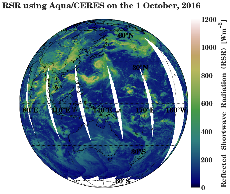
m = Basemap(projection='ortho', lon_0=140.714793, lat_0=-0.007606, resolution='c')
# c (crude) < l (low) < i (intermediate) < h (high) < f (full)
# Source: http://seesaawiki.jp/met-python/d/Basemap

X, Y = m(data_L1.lon.values, data_L1.lat.values)
VAL  = data_L1.rsr.values

m.scatter(X, Y, c=VAL, s=3.0, marker="s", zorder=1, vmin=0, vmax=1200, cmap=plt.cm.get_cmap('gist_earth'), alpha=1.0) 
m.colorbar(location='right', label='Reflected  Shortwave  Radiation  (RSR)  $\mathregular{[Wm^{-2}]}$')

m.drawcoastlines()
m.drawcountries()
m.drawmapboundary(fill_color='white')
m.drawparallels(np.arange(-60.,61.,30.),labels=[1,0,0,0],dashes=[2,2])
m.drawmeridians(np.arange(-160.,200.,30.),labels=[0,0,0,1],dashes=[2,2])
plt.title('RSR using Aqua/CERES on the 1 October, 2016  \n')

plt.annotate(u'60\N{DEGREE SIGN}S', xy=(m(170, -62.5)), color='black', fontweight='bold', xycoords='data', horizontalalignment='center', verticalalignment='top')
plt.annotate(u'30\N{DEGREE SIGN}S', xy=(m(170, -32.5)), color='black', fontweight='bold', xycoords='data', horizontalalignment='center', verticalalignment='top')
plt.annotate(u'30\N{DEGREE SIGN}N', xy=(m(170, +27.5)), color='black', fontweight='bold', xycoords='data', horizontalalignment='center', verticalalignment='top')
plt.annotate(u'60\N{DEGREE SIGN}N', xy=(m(170, +57.5)), color='black', fontweight='bold', xycoords='data', horizontalalignment='center', verticalalignment='top')
plt.annotate(u'80\N{DEGREE SIGN}E', xy=(m(80, -2.5))  , color='black', fontweight='bold', xycoords='data', horizontalalignment='center', verticalalignment='top')
plt.annotate(u'110\N{DEGREE SIGN}E', xy=(m(110, -2.5)), color='black', fontweight='bold', xycoords='data', horizontalalignment='center', verticalalignment='top')
plt.annotate(u'110\N{DEGREE SIGN}E', xy=(m(110, -2.5)), color='black', fontweight='bold', xycoords='data', horizontalalignment='center', verticalalignment='top')
plt.annotate(u'140\N{DEGREE SIGN}E', xy=(m(140, -2.5)), color='black', fontweight='bold', xycoords='data', horizontalalignment='center', verticalalignment='top')
plt.annotate(u'170\N{DEGREE SIGN}E', xy=(m(170, -2.5)), color='black', fontweight='bold', xycoords='data', horizontalalignment='center', verticalalignment='top')
plt.annotate(u'160\N{DEGREE SIGN}W', xy=(m(-160, -2.5)),color='black', fontweight='bold', xycoords='data', horizontalalignment='center', verticalalignment='top')
# plt.savefig("FIG/Scane_analysis_Aqua_CERES_RSR.png")
plt.show()

etc-image-3 — 그림. Aqua/CERES 기상위성 자료를 이용한 대기상단에서의 상향단파복사 가시화 (빈구).

[전체]

Sorry, something went wrong. Reload?

Sorry, we cannot display this file.

Sorry, this file is invalid so it cannot be displayed.

view raw Visualization_Using_NetCDF_Format_of_CERES_Data.ipynb hosted with ❤ by GitHub

참고 문헌

[논문]

없음

[보고서]

없음

[URL]

없음

문의사항

[기상학/프로그래밍 언어]

sangho.lee.1990@gmail.com

[해양학/천문학/빅데이터]

saimang0804@gmail.com

저작자표시 동일조건

'프로그래밍 언어 > Python' 카테고리의 다른 글

[Python] 파이썬 Spyder 편집기 소개 (0)	2020.11.02
[Python] 파이썬 원도우 (Window 10)에서 수치예측모델 (Grib, Grb2) 자료 처리를 위한 "wgrib, wgrib2, cdo" 설치 방법 (0)	2020.02.09
[Python] 파이썬 HDF 형식인 천리안위성 1A호 (COMS/MI) 기상위성 자료를 이용한 가시화 (4)	2019.10.23
[Python] 파이썬 Grib 및 Grb2 형식인 수치예측모델 (ECMWF) 자료를 이용한 가시화 (0)	2019.10.23
[Python] 파이썬 바이너리 형식인 히마와리 8호 (Himawari-8/AHI) 기상 위성 자료를 이용한 가시화 (0)	2019.10.22

내 블로그 - 관리자 홈 전환	`Q` `Q`
새 글 쓰기	`W` `W`

글 수정 (권한 있는 경우)	`E` `E`
댓글 영역으로 이동	`C` `C`

이 페이지의 URL 복사	`S` `S`
맨 위로 이동	`T` `T`
티스토리 홈 이동	`H` `H`
단축키 안내	`Shift` + `/` `⇧` + `/`