정보
-
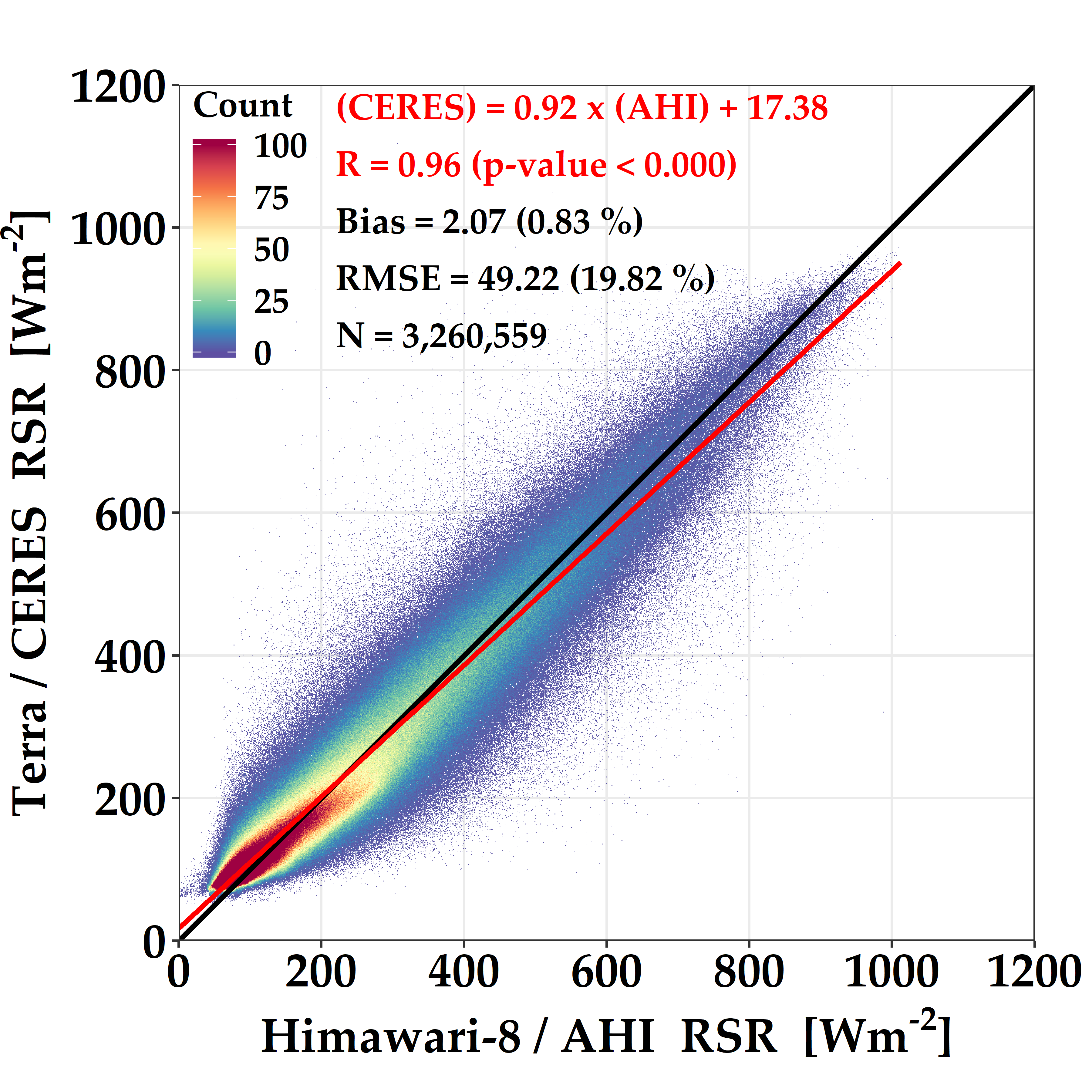
업무명 : 정지궤도/극궤도 기상위성으로부터 시공간 일치 자료 (Himawari-8/AHI vs Terra/CERES)를 이용한 2차원 빈도분포 산점도
-
작성자 : 이상호
-
작성일 : 2020-01-07
-
설 명 :
-
수정이력 :
내용
[특징]
-
Himawari-8/AHI 및 Terra/CERES의 시공간 일치 자료를 이해하기 위해서 가시화가 요구되며 이 프로그램은 이러한 목적을 달성하기 위한 소프트웨어
[기능]
-
시공간 일치 자료를 이용한 2차원 빈도분포 산점도
[활용 자료]
-
자료명 : Himawari-8/AHI (2 km) 및 Terra/CERES (20 km)의 시공간 일치 자료
-
자료 종류 : 대기상단에서의 상향단파복사 (RSR)
-
확장자 : ASCII 형태
-
기간 : 2015년 08월 15일 - 2017년 08월 15일 중에서 매월 15일
-
해상도 : 20 km
[자료 처리 방안 및 활용 분석 기법]
-
없음
[사용법]
-
입력 자료를 동일 디렉터리 위치
-
소스 코드를 실행 (Rscript 2D_Frequency_Scatter_Using_Spacetime_Coincidence_Data.R)
-
가시화 결과를 확인
[사용 OS]
-
Windows10
[사용 언어]
-
R v3.6.2
-
R Studio v1.2.5033
소스 코드
[명세]
-
전역 설정
-
최대 10 자리 설정
-
메모리 해제
-
# Set Option
options(digits = 10)
memory.limit(size = 9999999999999)
-
라이브러리 읽기
# Library Load
library(tidyverse)
library(RColorBrewer)
library(extrafont)
-
함수 선언
# Function Load
fnStatResult = function(xAxis, yAxis) {

   if (length(yAxis) > 0) {
      nSlope = coef(lm(yAxis ~ xAxis))[2]
      nInterp = coef(lm(yAxis ~ xAxis))[1]
      nMeanX = mean(xAxis, na.rm = TRUE)
      nMeanY = mean(yAxis, na.rm = TRUE)
      nSdX = sd(xAxis, na.rm=  TRUE)
      nSdY = sd(yAxis, na.rm = TRUE)
      nNumber = length(yAxis)
      nBias = mean(xAxis - yAxis, na.rm = TRUE)
      nRelBias = (nBias / mean(yAxis, na.rm = TRUE))*100.0
      # nRelBias = (nBias / mean(xAxis, na.rm = TRUE)) * 100.0
      nRmse = sqrt(mean((xAxis - yAxis)^2, na.rm = TRUE))
      nRelRmse = (nRmse / mean(yAxis, na.rm = TRUE)) * 100.0
      # nRelRmse = (nRmse / mean(xAxis, na.rm = TRUE)) * 100.0
      nR = cor(xAxis, yAxis)
      nMeanDiff = mean(xAxis - yAxis, na.rm = TRUE)
      nSdDiff = sd(xAxis - yAxis, na.rm = TRUE)
      nPerMeanDiff = mean((xAxis - yAxis) / yAxis, na.rm = TRUE) * 100.0
      nPvalue = cor.test(xAxis, yAxis)$p.value

      return( c(nSlope, nInterp, nMeanX, nMeanY, nSdX, nSdY, nNumber, nBias, nRelBias, nRmse, nRelRmse, nR, nMeanDiff, nPerMeanDiff, nPerMeanDiff, nPvalue) )
   }
}
-
자료 읽기
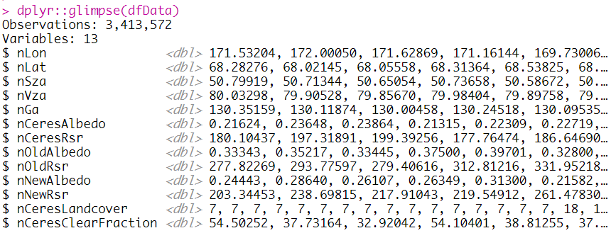
# Set Data Frame
dfData = data.table::fread("INPUT/Terra.OUT", header = FALSE)

colnames(dfData) = c("nLon", "nLat", "nSza", "nVza", "nGa", "nCeresAlbedo", "nCeresRsr", "nOldAlbedo", "nOldRsr", "nNewAlbedo", "nNewRsr", "nCeresLandcover", "nCeresClearFraction")

dplyr::glimpse(dfData)
-
Data Frame를 통해 L1 전처리
-
대기상단에서의 상향단파복사 (n*Rsr, 알베도 (n*Albedo), 태양 천정각 (nSza), 위성 천정각 (nVza), Sun glint (nGa)에 대한 최대값/최소값 설정
-
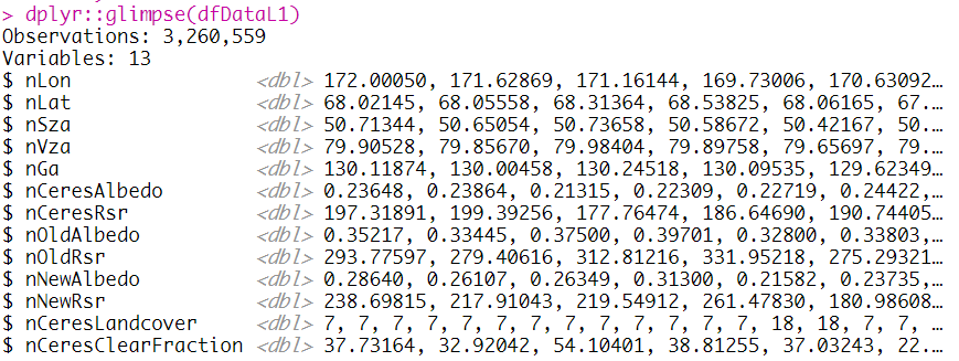
# L1 Processing Using Data Frame
dfDataL1 = dfData %>%
   dplyr::filter(
      dplyr::between(nCeresRsr, 0, 1400)
      , dplyr::between(nCeresAlbedo, 0, 1)
      , dplyr::between(nOldRsr, 0, 1400)
      , dplyr::between(nOldAlbedo, 0, 1)
      , dplyr::between(nNewRsr, 0, 1400)
      , dplyr::between(nNewAlbedo, 0, 1)
      , dplyr::between(nSza, 0, 80)
      , dplyr::between(nVza, 0, 80)
      , nGa >= 20
      )

dplyr::glimpse(dfDataL1)
-
가시화를 위한 초기 설정
# Set Value for Visualization
xAxis = dfDataL1$nNewRsr
yAxis = dfDataL1$nCeresRsr

xcord = 220
ycord = seq(1170, 0, -80)
cbSpectral = rev(RColorBrewer::brewer.pal(11, "Spectral"))
font = "Palatino Linotype"
nVal = fnStatResult(xAxis, yAxis)  ;  sprintf("%.3f", nVal)
-
ggplot2를 이용한 2차원 빈도분포 산점도
# Visualization Using ggplot2
ggplot() +
   coord_fixed(ratio = 1) +
   theme_bw() +
   stat_bin2d(aes(xAxis, yAxis), binwidth = c(1, 1)) +
   scale_fill_gradientn(colours = cbSpectral, limits = c(0, 100), na.value = cbSpectral[11]) +
   annotate("text", x = xcord, y = ycord[1], label = paste0("(CERES) = ", sprintf("%.2f", nVal[1])," x (AHI) + ", sprintf("%.2f", nVal[2])), size = 5, hjust = 0, color = "red", fontface = "bold", family = font) +
   # annotate("text", x = xcord, y = ycord[2], label =  "bold(R^\"2\" ~\"=\"~ \"0.914\"~\"(p-value < 0.001)\")", parse = TRUE, size = 5, hjust = 0, color = "red",family = font) +
   annotate("text", x = xcord, y = ycord[2], label = paste0("R = ", sprintf("%.2f", nVal[12]), " (p-value < ", sprintf("%.3f", nVal[16]), ")"), size = 5, hjust = 0, color = "red", family = font, fontface = "bold") +

   annotate("text", x = xcord, y = ycord[3], label = paste0("Bias = ", sprintf("%.2f", nVal[8]), " (", sprintf("%.2f", nVal[9])," %)"), parse = FALSE, size = 5, hjust = 0, family = font, fontface = "bold") +
   annotate("text", x = xcord, y = ycord[4], label = paste0("RMSE = ", sprintf("%.2f", nVal[10]), " (", sprintf("%.2f", nVal[11])," %)"), parse = FALSE, size = 5, hjust = 0, family = font, fontface = "bold") +
   annotate("text", x = xcord, y = ycord[5], label=paste0("N = ", format(nVal[7], big.mark = ",", scientific = FALSE)), size = 5, hjust = 0, color = "black", family = font, fontface = "bold") +
   geom_abline(intercept = 0, slope = 1, linetype = 1, color = "black", size = 1.0) +
   stat_smooth(aes(xAxis, yAxis), method = "lm", color = "red", se = FALSE) +
   scale_x_continuous(minor_breaks = seq(0, 1200, 200), breaks=seq(0, 1200, 200),  expand=c(0,0), limits=c(0,  1200)) +
   scale_y_continuous(minor_breaks = seq(0, 1200, 200), breaks=seq(0, 1200, 200),  expand=c(0,0), limits=c(0,  1200)) +
   labs(
      title = ""
      , x = expression(paste(bold("Himawari-8 / AHI  RSR  [Wm"^bold("-2")*"]")))
      , y = expression(paste(bold("Terra / CERES  RSR  [Wm"^bold("-2")*"]")))
      , fill = "Count"
      ) +
   theme(
      plot.title = element_text(face = "bold", size = 20, color = "black")
      , axis.title.x = element_text(face = "bold", size = 19, colour = "black")
      , axis.title.y = element_text(face = "bold", size = 19, colour = "black", angle = 90)
      , axis.text.x = element_text(face = "bold", size = 19, colour = "black")
      , axis.text.y = element_text(face = "bold", size = 19, colour = "black")
      , legend.title = element_text(face = "bold", size = 14, colour = "black")
      , legend.position = c(0, 1), legend.justification = c(0, 0.96)
      , legend.key=element_blank()
      , legend.text=element_text(size=14, face="bold")
      , legend.background=element_blank()
      , text=element_text(family=font)
      , plot.margin=unit(c(0,8,0,0),"mm")
      ) +
   ggsave(filename = paste0("FIG/Visualization_Using_ggplot2.png"), width = 6, height = 6, dpi = 1200)
[전체]
참고 문헌
[논문]
- 없음
[보고서]
- 없음
[URL]
- 없음
문의사항
[기상학/프로그래밍 언어]
- sangho.lee.1990@gmail.com
[해양학/천문학/빅데이터]
- saimang0804@gmail.com
'프로그래밍 언어 > R' 카테고리의 다른 글
| [R] 데이터 정제를 위한 "dplyr, tidyr" 패키지 소개 (0) | 2020.02.08 |
|---|---|
| [R] 기상 관측소 정보를 이용하여 태양 위치 시간 (일출/일몰/아침 골든/남중/저녁 골든/일몰/항해 박명/천문 박명/밤/아침 박명) 계산 (0) | 2020.01.09 |
| [R] 직달 일사량 자료를 이용한 일조량 산출 및 비교 분석 (0) | 2020.01.06 |
| [R] KLAPS 수치예측 모델 자료를 이용하여 내삽 방법 (Inverse Distance Weighting, Linear Interpolation)에 따른 전처리 및 가시화 (0) | 2020.01.03 |
| [R] 고층/상층 기상 자료 (라디오존데)를 이용한 전처리 및 단열선도 (Skew T Log P) 가시화 (0) | 2019.12.31 |


최근댓글